
Sensing Colour: The Bayer Mosaic, and What Interpolation Costs
Lesson 5 of Image Sensing. A silicon photosite is colourblind, so a mosaic of filters gives each one a single colour — a quarter red, a quarter blue, half green. Two thirds of every colour image is therefore interpolated, and measured against photosites that actually exist, that guess costs 4.7 DN on a flat patch and 129.9 DN at an edge: twenty-eight times worse where it shows.
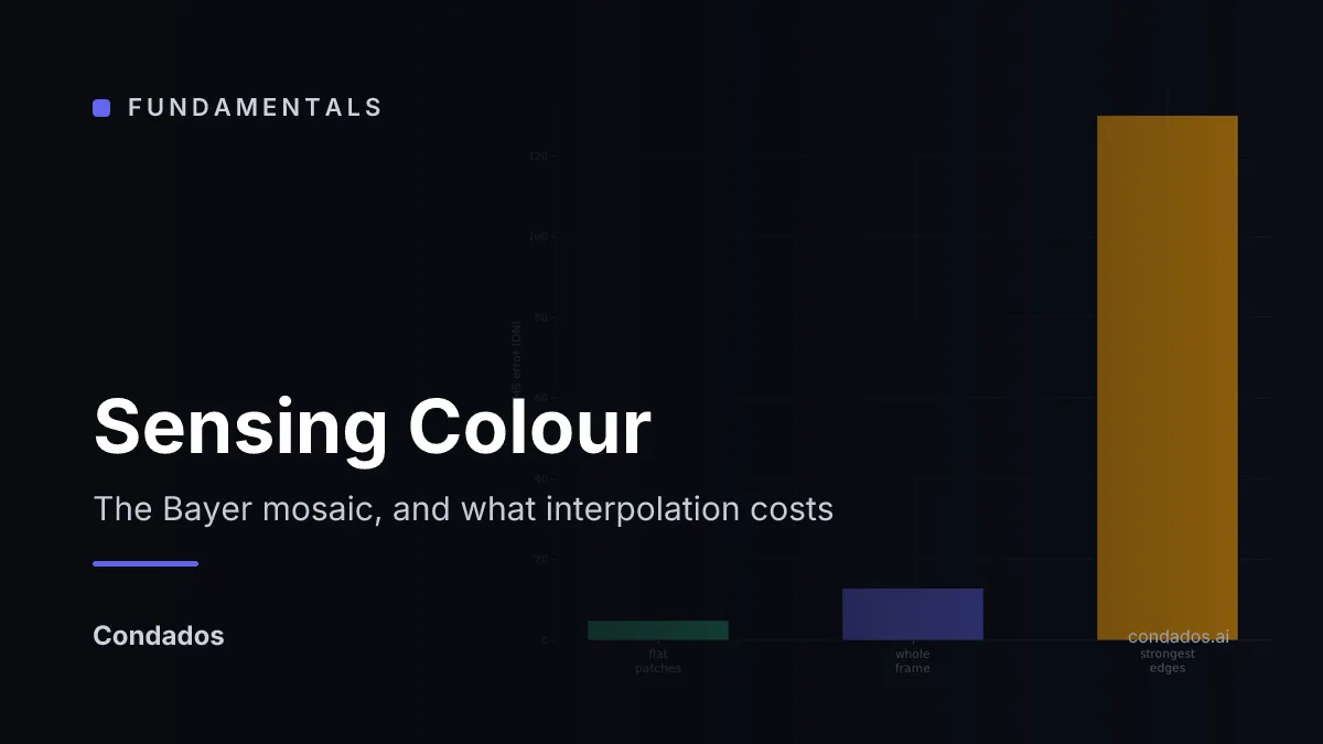
TL;DR — a silicon photosite counts photons and has no idea what colour they were. A mosaic of filters gives each one a single colour: a quarter red, a quarter blue, half green. So two thirds of every colour image is interpolated rather than measured — and against a reference built only from photosites that actually exist, that guess costs 4.7 DN on a flat patch and 129.9 DN at an edge. Twenty-eight times worse exactly where you can see it.
Where we are
Part of image sensing. Lesson 4 merged eighteen exposures into radiance and treated each channel as if it were simply there. This lesson is about where the three channels come from, and it is the last one in the unit.
One filter per photosite
Intuition: silicon responds to light across the whole visible range, so a bare photosite can tell you how much light arrived and nothing about its colour. The fix is brutally simple — put a coloured filter over each site and accept that each one now reports a single channel.
Bryce Bayer’s arrangement from 1976 [2] is still the one almost every camera uses: a repeating 2 × 2 cell with one red, one blue and two greens, because the eye resolves detail chiefly through the green-sensitive cones.
LibRaw reports this camera’s cell as [[0, 1], [3, 2]] against the channel description
RGBG — index 0 is red, 1 and 3 are the two greens, 2 is blue. Read off the grid, that
is RGGB: red top-left, green top-right, green bottom-left, blue bottom-right.
import cv2

# `raw` is a single-channel Bayer mosaic from the sensor.
# OpenCV names conversions by the opposite corner of the 2x2 cell, so an RGGB
# sensor is COLOR_BayerBG2BGR. Getting this wrong swaps red and blue and looks
# like a white-balance problem rather than a naming problem.
bgr = cv2.cvtColor(raw, cv2.COLOR_BayerBG2BGR)   # demosaic -> 3-channel BGR
#include <opencv2/opencv.hpp>
// `raw` is a single-channel Bayer mosaic. OpenCV names the conversion by the
// opposite corner of the 2x2 cell: an RGGB sensor is COLOR_BayerBG2BGR.
cv::Mat bgr;
cv::cvtColor(raw, bgr, cv::COLOR_BayerBG2BGR); // demosaic -> 3-channel BGRWhat the guess costs
Asserting that interpolation is “usually fine” is easy. Measuring it needs a reference that was never interpolated — and this unit’s scene [3] supplies one — and one is sitting inside the mosaic. Every 2 × 2 cell contains a real red, a real blue and two real greens, so binning the mosaic 2 × 2 gives a genuine colour image at half resolution with no guessing anywhere in it.
Demosaic at full resolution, bin the result the same way so both live on the same grid, and subtract:
| where | RMS error (DN, of 4095) |
|---|---|
| inside the chart’s flat patches | 4.686 |
| whole frame | 12.668 |
| the top 1% of gradient pixels | 129.928 |
| worst single value anywhere | 1437 |
What it means: on a flat patch the guess is worth about 4.7 DN, which against a 12-bit full scale of 4095 is around 0.1% — genuinely negligible, and it is why nobody notices demosaicing in a photograph of a wall. At the strongest 1% of edges it is 129.9 DN, twenty-eight times worse, and the worst single value is off by 1437 DN, a third of the entire range. Interpolation does not fail everywhere a little; it works almost perfectly nearly everywhere and then fails hard on exactly the boundaries an edge detector is about to look for.
Now you try
The crop below straddles the border between the chart’s blue patch and its green one. Step through what the sensor kept, what the demosaicer guessed, and what the guess got wrong.
Watch where the error concentrates. The flat interiors are almost perfect; the one-pixel boundary between the two patches is where the neighbours a demosaicer averages stop agreeing with each other. The lab’s own flat-and-edge numbers are not the table’s: it works on a 32-pixel crop with a plainer demosaicer and its own definition of an edge, so it reproduces the shape of the result and not its magnitude.
In the wild
The bench measurement showed the guess costing twenty-eight times more at an edge than on a flat patch. Here is the same asymmetry in a photograph, visible as colour rather than as a number in a table.
Comparing the local variation of red against blue — each channel high-passed, so the scene’s actual colour is removed and only the disagreement between channels remains — on a photograph of a red telephone box:
| mean red-minus-blue difference | |
|---|---|
| the strongest 1% of edges | 13.25 |
| the flattest half of the frame | 2.44 |
| ratio | 5.4× |
| worst single pixel | 150.5 |
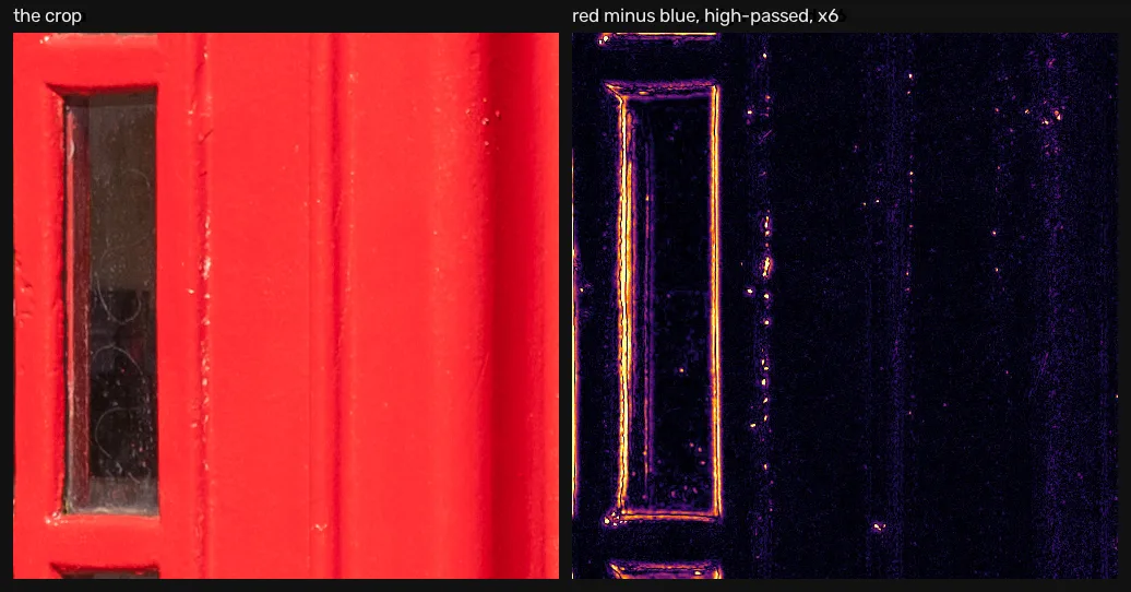
What it means: colour error in a photograph is an edge phenomenon, by a factor of five, exactly as the controlled measurement said it would be. One caveat this lesson owes you: demosaicing is not the only thing producing that fringe. A lens does not bring every wavelength to focus in the same plane either, and lateral chromatic aberration puts its error in the same places. This measurement cannot separate the two — it shows their sum, and separating them needs a lens model, which is unit 1.1’s business.
Where this breaks
The lab’s “original” is itself a demosaiced image, so it demonstrates the mechanism rather than measuring it. The numbers in the table above are the honest version, taken against 2 × 2 binning of the raw mosaic where every value is a photosite that existed.
Bilinear interpolation is the simplest demosaicer and the one measured here. Real converters use gradient-aware methods that are markedly better at exactly the edges where this one is worst, so 129.9 DN is an upper bound on a modern pipeline’s error, not a description of it. Testing that claim needs several demosaicers compared on the same frame, which this lesson did not do.
Two other things are named and not measured: a Bayer sensor cannot resolve fine alternating colour detail at all, which is where the coloured moiré on fabric comes from; and some sensors are not Bayer — X-Trans uses a 6 × 6 cell, and Foveon stacks three measurements at every position and has no demosaicing step at all.
Next
This closes unit 1.2. The three numbers at a pixel now exist, whatever their provenance — and The Image as Data picks them up: what array holds them, where its samples sit, how finely they are written, and what coordinate systems they can be written in.
Further reading
- Go deeper: Gonzalez & Woods, Digital Image Processing (4th ed.), ch. 7 (Color Image Processing, p. 529) [1] — §7.2 (Color Models, p. 535) picks up where this lesson stops.
- The original: Bayer’s patent [2] is three pages and the figure is the one every textbook redraws.
- Related on CondadosAI: from photons to counts — what the single value under each filter actually counts · colour, which takes these three numbers and asks what coordinates to put them in.
References
[1] Gonzalez, R. C., & Woods, R. E. (2018). Digital Image Processing (4th ed.), ch. 7 (Color Image Processing, p. 529), §7.2 (Color Models, p. 535). Pearson. Detailed table of contents.
[2] Bayer, B. E. (1976). Color imaging array. US Patent 3,971,065, filed 5 March 1975, granted 20 July 1976. Patent
[3] Fairchild, M. D. (2007). The HDR Photographic Survey. Proceedings of the IS&T 15th Color and Imaging Conference, pp. 233–238. doi:10.2352/CIC.2007.15.1.art00044 — the scene this unit measures. Used for research and non-commercial publication, as its terms require; images are downloaded, never redistributed.