The Pinhole Model: Why a Hole Makes a Picture, and Where the Prediction Fails

Lesson 1 of the Image Formation unit. A pinhole projects a scene point to a pixel by similar triangles, and that is a prediction you can check. Worked on one board corner from OpenCV's calibration set: the model puts it at (523.98, 77.94) and the detector found it at (513.77, 86.53), 13.34 px apart. Across the view the error is 0.29 px in the middle third of the frame and 5.75 px in the outer third, which is the shape of the problem the rest of the unit solves.

Luis Condados · August 19, 2026

computer-vision camera-calibration optics fundamentals

How far the straight-line model misses, against how far from the optical axis the point sits. Flat in the middle of the frame, steep at the edges.

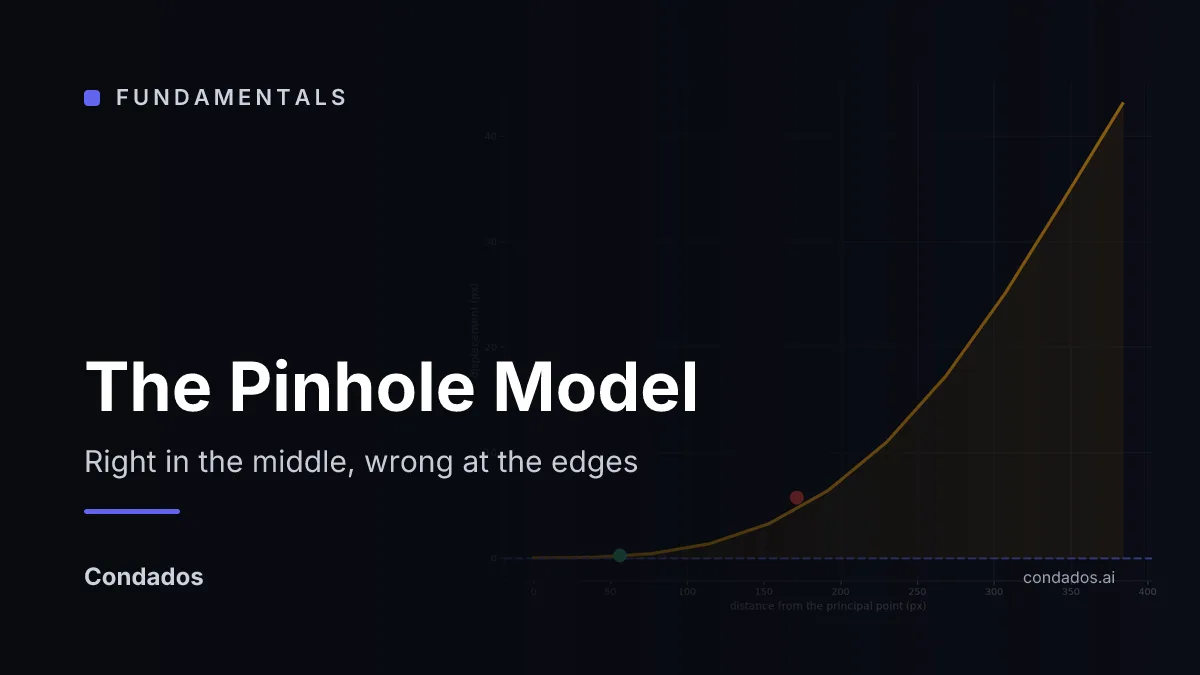
A pinhole camera is similar triangles and nothing else: a point at distance $Z$ and offset $X$ lands at $fX/Z$ on the sensor. That is a prediction, so it can be checked. On one photograph from OpenCV’s calibration set the model puts a board corner at (523.98, 77.94) and the detector found it at (513.77, 86.53), a gap of 13.34 px. The gap is not spread evenly: 0.29 px for corners near the middle of the frame and 5.75 px for corners near its edges.

Where we are

Lesson 1 of image formation. Nothing on the track comes before it. The unit’s job is to explain how a three-dimensional scene becomes a grid of numbers, and the first question is why any of it is sharp.

A hole is a filter on rays

Point a bare sensor at a room and every photosite receives light from everywhere. Each cell sums the whole room, so the result is a uniform grey with no picture in it. Put a barrier with a small hole in front, and each point on the sensor can only be reached from one direction. That restriction is what makes an image: the hole turns “light from the whole room” into “light from one direction per pixel” [1].

Once each pixel corresponds to one ray, the geometry is a pair of similar triangles. A point sitting $X$ to the side at depth $Z$ projects onto the image plane at distance $f$ behind the hole, and the two triangles share an angle:

\frac{x}{f} = \frac{X}{Z}, \qquad \frac{y}{f} = \frac{Y}{Z}.

Sensors are indexed in pixels rather than millimetres, and the optical axis does not necessarily meet the sensor at its middle. Writing the focal length in pixels as $f_x, f_y$ and the point where the axis crosses the sensor as $(c_x, c_y)$ :

u = c_x + f_x\frac{X}{Z}, \qquad v = c_y + f_y\frac{Y}{Z}.

Two scalar equations, one division each. Every camera model in computer vision is built on top of these [2], and the rest of this unit is about the ways a real camera departs from them.

The two triangles meet at the hole and share an angle, so their sides are in the same ratio: x / f = X / Z. Drawing the image plane in front of the hole rather than behind it avoids the upside-down image and changes nothing else.

Checking it on a real corner

The unit’s camera comes from 13 photographs of a printed chessboard [4], which give $f_x = 536.07$ , $f_y = 536.02$ and a principal point at (342.37, 235.54). Note that the principal point is 22 px right of the frame’s centre; the optical axis and the middle of the sensor are not the same place, and assuming they are would put every prediction below 22 px off before it started.

Calibration also recovers where the board was in each shot. Take that as given for now, since recovering pose is unit 4.1’s subject, and look only at what happens after: a corner whose position in the camera’s own frame is known, projected by the two equations above.

Worked example · One corner of the board in left01.jpg

The corner at the far end of the board’s long edge sits, in the camera’s frame, at

(X, Y, Z) = (4.6866,\; -4.0674,\; 13.8341)

in board units. Substituting into the two equations:

u = 342.37 + 536.07 \times \frac{4.6866}{13.8341} = 342.37 + 181.61 = 523.98

v = 235.54 + 536.02 \times \frac{-4.0674}{13.8341} = 235.54 - 157.60 = 77.94

The corner detector, working on the pixels alone, puts that same corner at (513.77, 86.53).

What it means: the prediction is off by 13.34 px. On a 640×480 frame that is about 2% of the width, which is far too much to call agreement, and it is the largest error in this view. The model is not broken, though: this corner sits 227 px from the principal point, out where the departure lives.

Averaged over all 54 corners in that photograph, the pinhole equations miss by 2.55 px. Splitting the corners by how far they sit from the principal point shows what that average is hiding:

Corners	Mean distance from the principal point	Mean error
Innermost third	56 px	0.29 px
Outermost third	171 px	5.75 px

Near the middle of the frame the model is right to about a quarter of a pixel. Out at the edges it is twenty times worse. Whatever is wrong grows with distance from the centre, which is a strong hint about its cause and the subject of lesson 3.

Written out, the prediction is two lines of arithmetic:

# (X, Y, Z) is the corner in the camera's own frame; fx, fy, cx, cy from calibration.
u = cx + fx * X / Z
v = cy + fy * Y / Z

// (X, Y, Z) is the corner in the camera's own frame; fx, fy, cx, cy from calibration.
const double u = cx + fx * X / Z;
const double v = cy + fy * Y / Z;

What perspective does to a scene

Because the division is by $Z$ , two things follow that the human eye takes for granted. An object twice as far away covers half as many pixels, so size on the sensor carries distance. And lines that are parallel in the world stop being parallel in the image unless they are parallel to the sensor, because each point along them is divided by a different $Z$ .

The same division is why one photograph cannot tell you how big anything is: doubling both an object’s size and its distance leaves $X/Z$ unchanged, so a small near object and a large far one produce identical pixels.

Now you try

Move the ball and the camera and watch the projected position follow the two equations. Then switch to the second panel, which holds $X/Z$ fixed while changing both: two very different scenes, one photograph.

Try it: the red-ball scene in 3-D

Scene drag to orbit · scroll to zoom

What the camera sees the render (640×480)

In the wild

The pinhole model’s central claim is that parallel lines in the world meet at a single point in the image. That is testable on any photograph with architecture in it, and it does not need a calibration target.

A temple cloister, shot straight down its axis. Detect line segments with OpenCV’s own Hough transform [3], keep the 60 longest that are neither vertical nor horizontal — those are the receding ones, since a building’s own uprights meet only at infinity — and find the point that is closest to all of them at once.


segments detected	631
long receding lines kept	60, from 305 to 523 px
after one outlier pass	53
vanishing point	(872, 1076) px, inside the frame
median distance from a line to that point	45.1 px
as a fraction of the frame diagonal	1.6%

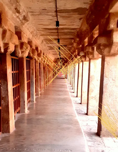
A temple cloister with 60 detected lines drawn over it, all converging on a marked point at the end of the corridor — The lines that were fitted, and the point they agree on. Nobody told the algorithm where the corridor ends. Source: “The Cloister Mandapam, in One point perspective” by Sindugab (Wikimedia Commons), CC0.

What it means: 53 lines from stone that was cut by hand, photographed on a phone, agree on one point to within 1.6% of the frame. That residual is not the model failing — it is the masonry not being perfectly straight, the lens not being perfectly rectilinear, and the segments being fitted to a few hundred pixels each. The projection this lesson derives from a hole in a box survives contact with a real building.

Where this breaks

The error is radial, and it is not small. The table above is the failure: 0.29 px in the middle of the frame against 5.75 px at the edges, with a worst corner 13.34 px out. Adding the lens terms that lesson 3 covers drops the same view’s mean error from 2.55 px to 0.170 px, with a worst corner of 0.404 px. The pinhole equations are not an approximation that gets uniformly better with care; they are missing a term that only matters away from the axis.

Depth is gone and cannot be recovered from one image. The projection maps a three-dimensional world onto two dimensions, and the information lost is not retrievable by looking harder. Everything the geometry branch of this track does later, from stereo to structure from motion, exists to put it back.

And a pinhole sharp enough for this is too dark to use. The whole model above assumes each pixel sees exactly one ray, which requires a hole of essentially no size. A hole of no size passes no light, so the exposure time runs to minutes and anything that moves is a smear. Open the hole to get light back and each sensor point starts collecting a cone of rays instead of one, which is blur. That trade is not a detail of construction. It is the reason no camera you own is a pinhole camera.

A lens collects a wide cone of light and bends it back to a point, buying the brightness a pinhole cannot have. It charges for it with a plane of focus, and lenses, focal length and depth of field is about what exactly is in focus once you have one.

Run it: every code block on this page has a cell in the unit’s notebook — open it in Colab.

References

[1] Forsyth, D. A., & Ponce, J. (2012). Computer Vision: A Modern Approach (2nd ed.), ch. 1 “Geometric Camera Models”, §1.1.1 “Pinhole Perspective” (p. 4). Pearson.

[2] Hartley, R., & Zisserman, A. (2004). Multiple View Geometry in Computer Vision (2nd ed.), ch. 6 “Camera Models” (p. 153). Cambridge University Press.

[3] OpenCV Documentation (5.0). Camera calibration and 3D reconstruction. docs.opencv.org/5.0

[4] Zhang, Z. (2000). A flexible new technique for camera calibration. IEEE Transactions on Pattern Analysis and Machine Intelligence, 22(11), 1330–1334. doi:10.1109/34.888718

Tagged