Corners: The Structure Tensor, Harris, Shi-Tomasi and Förstner

Lesson 5 of the Edge Detection unit. A contour says where a boundary runs but not where you are along it. Two eigenvalues of a 2x2 matrix fix that: measured on a real photo, flat background scores 0.001/0.000, an edge 0.411/0.019 and a corner 0.442/0.318. Harris, Shi-Tomasi and Förstner all read that same matrix, and on the edge patch Harris comes out positive at k = 0.04 and negative at k = 0.06, so k decides the answer rather than the data.

Luis Condados · August 18, 2026

computer-vision image-processing edge-detection harris features fundamentals

The strongest Harris responses on the same frame. They land where two edges meet, which is the one place a contour cannot tell you where you are.

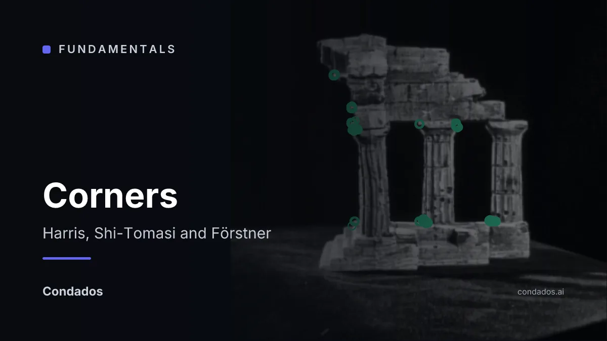
Every operator so far returns curves, and a curve cannot tell you where you are along it. The fix is to ask whether brightness changes in both directions rather than one, which is false along a column edge and true where it meets the base. Measured on the canonical frame, flat background scores eigenvalues 0.001 / 0.000, an edge 0.411 / 0.019 and a corner 0.442 / 0.318. Harris, Shi-Tomasi and Förstner all read that one matrix. On the edge patch Harris is positive at k = 0.04 and negative at k = 0.06, so on that patch the constant decides the answer, not the image.

Where we are

Lesson 4 ended on two limits with one cause. Non-maximum suppression fails at a junction because “the gradient direction” is not defined there, and every contour it produces is a curve, so two photographs of the same temple give two sets of curves with no way to pair up points on them.

Both come from asking a one-directional question. A column’s silhouette is an edge because brightness changes across it. Along it nothing changes at all, which is why you cannot say how far up the column you are. So ask about both directions.

Flat, edge, or corner: two eigenvalues decide

Slide the window one pixel in every direction and ask how much the content changes. A patch is matchable when it changes a lot in every direction. The object that captures this is built from the image gradients $I_x$ and $I_y$ (how fast brightness changes horizontally and vertically), averaged over the window $W$ :

M \;=\; \frac{1}{|W|}\sum_{(x,y)\in W} \begin{bmatrix} I_x^2 & I_x I_y \\ I_x I_y & I_y^2 \end{bmatrix}

The two eigenvalues $\lambda_1 \ge \lambda_2$ of $M$ measure the gradient energy along the two principal directions of the patch. The classification, due to Harris and Stephens [1] and covered in Szeliski §7.1.1 (Feature detectors) [5]:

$\lambda_1$	$\lambda_2$	patch	in the patio
small	small	flat	the black backdrop
large	small	edge	a column’s silhouette
large	large	corner	where the base meets a column

Worked example · Three 4×4 toy patches, by hand

Work on 4×4 patches of intensities in $\{0, 1\}$ , with central-difference gradients $I_x = (I_{right} - I_{left})/2$ on the four interior pixels.

Edge (dark left half, bright right half; every row is 0 0 1 1): each interior pixel has $I_x = (1-0)/2 = 0.5$ and $I_y = 0$ , so

M = \begin{bmatrix} 0.25 & 0 \\ 0 & 0 \end{bmatrix} \;\Rightarrow\; \lambda_1 = 0.25,\; \lambda_2 = 0

Corner (bright bottom-right quadrant): the four interior gradients are $(0,0)$ , $(0,0.5)$ , $(0.5,0)$ , $(0.5,0.5)$ . Averaging their outer products:

M = \begin{bmatrix} 0.125 & 0.0625 \\ 0.0625 & 0.125 \end{bmatrix} \;\Rightarrow\; \lambda_{1,2} = 0.125 \pm 0.0625 = 0.1875,\; 0.0625

Flat (all zeros): $M = 0$ , so $\lambda_1 = \lambda_2 = 0$ .

What it means: the edge has all its energy on one axis ( $\lambda_2 = 0$ says sliding along the edge costs nothing, the aperture problem in one number). The corner resists sliding on both axes. The flat patch resists nothing.

The same computation on the real photo [6], with Sobel gradients and a 21×21 window (these three spots are the presets in the lab below; artifact output/sift_numbers.json):

spot on the temple photo	$\lambda_1$	$\lambda_2$	verdict
background (50, 60)	0.001	0.000	flat
column silhouette (277, 240)	0.411	0.019	edge
base corner (150, 320)	0.442	0.318	corner

The ratio between the cases is enormous: the edge carries 22× more energy in its first direction than its second (0.411 / 0.019), while the corner is within a factor of 1.4 of isotropic. No tuned threshold is needed to tell these apart.

The three cases as gradient pictures. An edge’s gradients all point across it, so one eigenvalue collects everything and sliding along the edge is free. A corner’s gradients disagree, and that disagreement is what makes it findable. The numbers under each panel are measured on the temple photo.

Now you try

Drag the window over the photo and watch the eigenvalues respond; the three dots mark the preset spots from the table. The right panel scatters every pixel’s $(I_x, I_y)$ pair: an edge collapses the scatter onto a line, a corner spreads it, and the ellipse (axes $\sqrt{\lambda_1}, \sqrt{\lambda_2}$ ) summarizes the shape.

Try it: drag the window — flat, edge, or corner?

Try the silhouette of a column, then slide along it. The verdict stays “edge” and the ellipse stays needle-shaped the whole way down, which is the aperture problem made visible: the patch cannot tell you where along the edge it came from.

Three responses, one matrix

Computing two eigenvalues per pixel was expensive in 1988, and all three classical detectors avoid it by scoring the matrix directly. They differ in what they consider a corner, and all three are still the standard entry points into feature extraction [4].

Harris and Stephens [1] use the determinant and trace, which are $\lambda_1\lambda_2$ and $\lambda_1 + \lambda_2$ and cost no eigendecomposition:

R = \det M - k\,(\operatorname{tr} M)^2

Shi and Tomasi [2] take the smaller eigenvalue on its own, $\min(\lambda_1, \lambda_2)$ , on the grounds that a patch is only as trackable as its weakest direction.

Förstner and Gülch [3] refuse to collapse the two into one number. They report a strength, $w = \det M / \operatorname{tr} M$ , and separately a roundness, $q = 4\det M / (\operatorname{tr} M)^2$ , which is 1 for a perfectly isotropic patch and 0 for a pure edge.

Worked example · The three measured spots, scored three ways

The eigenvalues measured above, put through each response:

spot	$\lambda_1$	$\lambda_2$	$R$ (k=0.04)	$R$ (k=0.06)	Shi-Tomasi	$w$	$q$
background	0.001	0.000	-0.000000	-0.000000	0.000	0.00000	0.0000
column edge	0.411	0.019	+0.000413	-0.003285	0.019	0.01816	0.1689
base corner	0.442	0.318	0.117452	0.105900	0.318	0.18494	0.9734

Substituting for the corner at k = 0.04:

R = (0.442)(0.318) - 0.04\,(0.442 + 0.318)^2 = 0.140556 - 0.023104 = 0.117452

What it means: all three agree the corner is a corner and the background is nothing. They disagree about the edge, and the disagreement is instructive.

Harris separates corner from edge by a factor of 284, far more than Shi-Tomasi’s 16.7, so as a ranking it is the sharper of the two. But its edge score at k = 0.04 is positive. Any pipeline that keeps pixels where $R > 0$ accepts that edge patch as a corner. Raise k to 0.06 and the same patch scores -0.003285 and is rejected. The constant is doing the deciding, on real numbers, which is why k is quoted as a range and not a value.

Shi-Tomasi has no constant to get wrong; 0.019 against 0.318 needs no interpretation. Förstner’s $q$ says the same thing on a scale that is free of contrast entirely: 0.1689 for the edge against 0.9734 for the corner, where 1 would be a perfectly round error ellipse.

In the wild

A detector that finds six hundred corners is worth nothing if they are six hundred different corners each time the camera moves. The property that matters is repeatability, and it can be measured on any photograph by rotating it and asking how many points come back.

Detecting Harris corners on a market stall, rotating the image by a known angle, detecting again, mapping those detections back, and counting a corner as repeated when some detection lands within three pixels of it:

rotation	corners in the interior	repeated within 3 px	repeatability
5°	374	319	85.3%
15°	374	331	88.5%
45°	374	318	85.0%

A market fruit stall with several hundred detected corners marked, clustered on the fruit boundaries and the stall structure — Where the detector puts its points: on the boundaries between fruit, on the crate edges, on the lettering. Source: “Marrakech souk fruit vendor” by Mustang Joe (Wikimedia Commons), CC0.

What it means: between 85% and 88% of interior corners survive a rotation, and the figure barely moves between 5° and 45°. That is the rotation invariance this lesson derives from the structure tensor’s eigenvalues, confirmed on a photograph nobody prepared — a rotated eigenvalue pair is the same eigenvalue pair, so the corner measure does not care which way the camera was held.

Two honest notes. The one-in-seven that does not come back is mostly interpolation: the rotation resamples the image, which moves weak corners by more than three pixels or softens them below the detector’s quality threshold. And 15° scoring higher than 5° is noise, not a trend — three rotations of one image cannot resolve a two-point difference, and reading a mechanism into it would be exactly the mistake this site’s own rules warn about.

Where this breaks

The window is a fixed size. Every number above came from a 21x21 patch, and that choice is baked into the answer.

The base corner fills a 21x21 window at the distance this photograph was taken. Move the camera to a third of that distance and the same corner spans sixty pixels, so the window now sits entirely inside one straight run of the base and reports an edge. The corner did not change. The question did.

This is not a threshold problem and no response function fixes it, because all three read a matrix that was already built at one scale. A detector tied to one window size finds features of one size, and two photographs taken from different distances will not agree on a single point.

The second limit is subtler and shows in the lab above: a corner is found to the pixel, and a pixel is not a description. Two corners that look identical to the structure tensor are indistinguishable, so even a repeatable detector gives you nothing to match with.

Both are where the next unit starts. Searching for the same feature across a range of window sizes is what a scale space is for, and summarising a patch as a vector of numbers is what a descriptor is. SIFT does both [7], and it opens on the eigenvalue test above, at every scale at once.

That closes the Edge Detection unit: from what counts as an edge, through the two derivatives that find one, to Canny’s repair, and finally to the points that survive being looked at twice.

References

[1] Harris, C. G., & Stephens, M. (1988). A Combined Corner and Edge Detector. Proceedings of the Alvey Vision Conference 1988, pp. 1-6. doi:10.5244/C.2.23

[2] Shi, J., & Tomasi, C. (1994). Good features to track. CVPR 1994, pp. 593-600. doi:10.1109/CVPR.1994.323794

[3] Förstner, W., & Gülch, E. (1987). A Fast Operator for Detection and Precise Location of Distinct Points, Corners and Centres of Circular Features. Proceedings of the ISPRS Conference on Fast Processing of Photogrammetric Data, Interlaken, pp. 281-305. No DOI is published for this paper.

[4] Gonzalez, R. C., & Woods, R. E. (2018). Digital Image Processing (4th ed.), ch. 12 “Feature Extraction”. Pearson. Chapter title verified against the publisher’s detailed table of contents; no section-level locator is quoted here because none was checked.

[5] Szeliski, R. (2022). Computer Vision: Algorithms and Applications (2nd ed.), ch. 7 “Feature Detection and Matching”. Springer. Free PDF

[6] Seitz, S. M., Curless, B., Diebel, J., Scharstein, D., & Szeliski, R. (2006). A Comparison and Evaluation of Multi-View Stereo Reconstruction Algorithms. CVPR 2006, pp. 519-528. doi:10.1109/CVPR.2006.19 — the Middlebury multi-view datasets: vision.middlebury.edu/mview

[7] Lowe, D. G. (2004). Distinctive Image Features from Scale-Invariant Keypoints. International Journal of Computer Vision, 60(2), 91-110. doi:10.1023/B:VISI.0000029664.99615.94

Tagged