
Sensor Noise and Dynamic Range: Measuring the Gain You Were Never Told
Read the same photosite three times and you get three numbers. Plotting the variance of a count against its mean gives a straight line whose slope is the sensor's gain: 0.294 DN per electron on this camera, R² = 0.986, a full well of 13,199 electrons and at least 11.21 stops of dynamic range — none of which appears anywhere in the file.
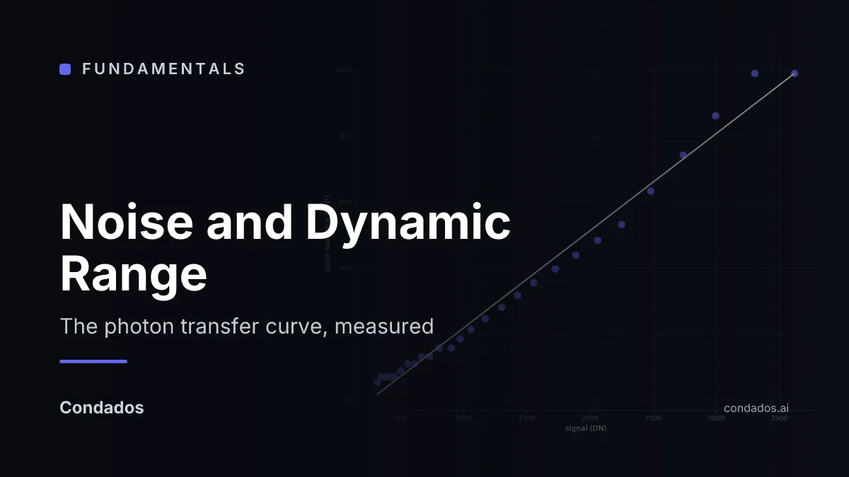
A count is a random variable. Most of its randomness is the light itself: photons arrive independently, so a well holding electrons has a standard deviation of electrons, and nothing about the camera can change that. Plot variance against signal and the line’s slope is the gain the manufacturer never wrote down — 0.294 DN per electron here, meaning one digital number is 3.4 electrons, the well holds 13,199 of them, and the sensor spans at least 11.21 stops.
Where we are
Lesson 2 of image sensing. Lesson 1 left a count as a number proportional to light times exposure, with a gain nobody had measured. This lesson measures it, and the measurement only needs one thing the scene happens to provide: three frames taken at the same settings. The bracket ends with three 30 s exposures because the camera reached its shutter limit and the photographer kept going [3].
Two kinds of noise, and only one of them is the camera’s fault
Shot noise is the light. Photons arrive as a Poisson process, so if a photosite collects electrons on average, the number it actually collects varies with variance . Its standard deviation is : quadruple the light and the noise only doubles, which is why bright pictures look clean and dark ones do not.
Read noise is the electronics: the amplifier, the converter, the wiring. It adds a roughly constant spread that does not care how much light arrived. In the dark it is all you have. The pair of them is the Poissonian-Gaussian model that denoising work fits to raw data [2].
Together, in electrons:
Counts are electrons times the gain , and variances scale by the square of a factor, so in the numbers you can actually see:
That is a straight line in a plot of variance against mean. Its slope is the gain in DN per electron and its intercept is the read noise squared. Measuring a sensor is plotting that line, and it is what the EMVA 1288 standard formalises for industrial cameras [4]. Healey and Kondepudy set the same model out for computer vision thirty years ago [1].
Variance in time, not in space
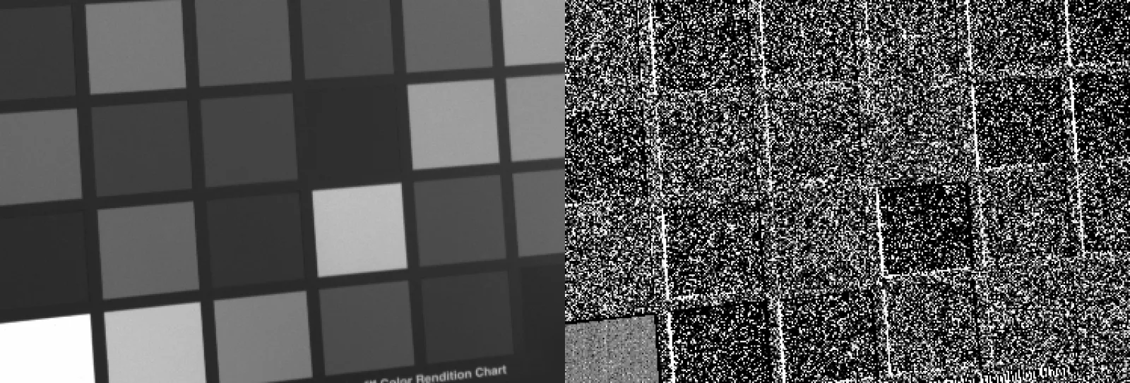
The catch is what “variance” means. Take one frame and compute the spread of a patch of it and you measure the paint, the lighting gradient and the dust, not the sensor. The spread has to come from repeated frames of the same thing, pixel by pixel:
import numpy as np

# three exposures of the same scene at the same shutter speed, one colour channel
stack = np.stack([green(a), green(b), green(c)]).astype(np.float64)
mean = stack.mean(axis=0)

# variance from the median absolute deviation of frame differences: robust to the
# pixels that differ for reasons that are not noise, and exact for Gaussian noise
differences = np.concatenate([(stack[0] - stack[1]).ravel(),
                              (stack[0] - stack[2]).ravel(),
                              (stack[1] - stack[2]).ravel()])
sigma_difference = np.median(np.abs(differences)) / 0.6745
variance = sigma_difference ** 2 / 2
// The same estimator with OpenCV: differences of repeats, then a robust spread.
cv::Mat diff, absdiff;
cv::subtract(frameA, frameB, diff, cv::noArray(), CV_64F);
absdiff = cv::abs(diff);
std::vector<double> values(absdiff.begin<double>(), absdiff.end<double>());
std::nth_element(values.begin(), values.begin() + values.size() / 2, values.end());
double sigmaDifference = values[values.size() / 2] / 0.6745;
double variance = sigmaDifference * sigmaDifference / 2.0;Three frames give a variance with two degrees of freedom, which is a wobbly thing: its sample median sits about 30% below the true value and its sample mean is dragged up by every pixel where the frames differ for a reason that is not noise. The median absolute deviation of the differences avoids both, and the artifact records the other estimator beside it as a check. On the green channel they land at 0.294 and 0.292 DN per electron, so the choice of estimator is not what the result rests on.
The measurement
Read noise, and why this scene cannot measure it
The three repeated frames are 30 s exposures. At 30 s nothing in this scene is dark: the faintest usable signal is 317 DN, which is a thousand electrons, whose shot noise alone is 33 times bigger than any plausible read noise. Extending the fitted line back to zero from there is an extrapolation across three hundred DN of nothing, and the negative intercept is the honest consequence.
So the read noise here is a bound, from a different frame: the darkest corner of the 1/800 s exposure, where the scene contributes almost nothing.
| Channel | dark corner | in electrons | full well | dynamic range |
|---|---|---|---|---|
| red | 1.90 DN | 5.6 e⁻ | 11,992 e⁻ | ≥ 11.07 stops |
| green | 1.64 DN | 5.6 e⁻ | 13,199 e⁻ | ≥ 11.21 stops |
| blue | 1.74 DN | 4.8 e⁻ | 11,180 e⁻ | ≥ 11.20 stops |
That spread includes fixed-pattern non-uniformity, dark current and any stray light that reached the corner, so it can only be too large, never too small. Dynamic range computed from it,
is therefore a lower bound as well. Quoting it as “11.21 stops” without the word “bound” would be the kind of number that survives a spot check and is still wrong.
Now you try
Set a gain and a read noise, then let the lab measure them back from simulated frames. Turn shot noise off and the line goes flat: the slope exists because light arrives at random.
The lab starts at 20 e⁻ of read noise, which is more than this sensor has, so that the intercept is visible at all. Pull it down towards the 5.6 e⁻ measured above and watch the intercept sink into the fit’s own scatter until it reads “not measurable” — which is the position this lesson is in, and why the dynamic range above is a bound.
In the wild
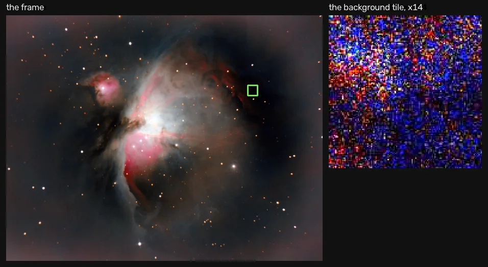
The same photograph, asked the other question. That background tile does not just have a mean of 3.35 — it has a standard deviation of 3.35 as well.
What it means, and the first number is the interesting one. In the empty sky the noise is as large as the signal: mean 3.35, sigma 3.35. That region carries no information at all — it is the floor this lesson has been measuring, seen in a photograph somebody took for its own sake. Everything the picture actually shows sits in the 6.25 stops above it.
Compare that with the 11.1 stops measured on the bench earlier in this lesson. The difference is not that this camera is worse. It is that the bench measured a raw frame against its own read noise, and this is an 8-bit JPEG that has already been developed, curved and quantized. The dynamic range a sensor has and the dynamic range that survives to the file you open are two different numbers, and the second one is always smaller.
Where this breaks
- ISO is fixed at 100 in every frame of this bracket. Raising ISO raises the analog gain before the converter, so it changes and leaves the electrons alone. That is why a high-ISO photograph is noisier but not because “ISO adds noise” — it amplifies a signal that was already too small. This scene cannot show it, and this lesson does not pretend to have measured it.
- Three repeats is thin. Each variance has two degrees of freedom; only pooling thousands of pixels per bin makes the curve stable. A proper characterisation uses dozens of frames per level and a uniformly lit target [4].
- The scene is not a flat field. The bins pool pixels from wherever the frame happens to be at that level, so texture, flare and dust all get a vote. The ColorChecker patches are the clean version of the same measurement and they agree, which is the reassurance available here.
- “Noise” in the restoration literature means something else. Gonzalez and Woods catalogue noise by its probability density — Gaussian, Rayleigh, salt-and-pepper [5] — which is the right vocabulary for a filter and the wrong model for a sensor. Shot noise is not an additive nuisance; it is the signal.
- Fixed-pattern noise is invisible to this method. Variance in time removes anything that repeats from frame to frame, which is exactly what fixed pattern is. It is real, it is in your images, and the number above does not include it.
- The gain differs per channel — 0.294 (green), 0.342 (red), 0.366 (blue) DN per electron — so there is no single “the gain” for this sensor. The channels are also scaled relative to each other somewhere before the file is written, which is consistent with that spread; this unit measures the spread and does not test which stage produces it.
Next
The counts in this lesson are proportional to light, and every number came out of the raw file. Open the same photograph as a JPEG and none of that holds: lesson 3 measures the curve that sits between them, and names the algorithms it breaks.
References
[1] Healey, G. E., & Kondepudy, R. (1994). Radiometric CCD camera calibration and noise estimation. IEEE Transactions on Pattern Analysis and Machine Intelligence, 16(3), 267–276. doi:10.1109/34.276126
[2] Foi, A., Trimeche, M., Katkovnik, V., & Egiazarian, K. (2008). Practical Poissonian-Gaussian Noise Modeling and Fitting for Single-Image Raw-Data. IEEE Transactions on Image Processing, 17(10), 1737–1754. doi:10.1109/TIP.2008.2001399
[3] Fairchild, M. D. (2007). The HDR Photographic Survey. Proceedings of the IS&T 15th Color and Imaging Conference, pp. 233–238. doi:10.2352/CIC.2007.15.1.art00044 — the scene, and the three 30 s frames this lesson depends on. Used for research and non-commercial publication, as its terms require.
[4] European Machine Vision Association (2021). EMVA Standard 1288, Release 4.0 Linear: Standard for Characterization of Image Sensors and Cameras, effective 21 June 2021. emva.org
[5] Gonzalez, R. C., & Woods, R. E. (2018). Digital Image Processing (4th ed.), ch. 5 “Image Restoration and Reconstruction”, §5.2 “Noise Models”, p. 366. Pearson.