The Laplacian, LoG and Zero-Crossings

Lesson 3 of the Edge Detection unit. The second derivative crosses zero at an edge instead of peaking, which locates a step edge at exactly x = 3.5 from integer pixels. It also has no smoothing in it: nine pixels disturbed by 0.03 produce four sign changes where there should be one. Measured on a photo, noise multiplies the zero-crossing pixels by 2.76x at sigma = 1.0 and 1.02x at sigma = 3.0, and only 33% of the resulting contours are closed.

Luis Condados · August 18, 2026

computer-vision image-processing edge-detection laplacian fundamentals

LoG zero-crossings at sigma 1, 2 and 3. More smoothing means less structure, and less of it invented by noise.

A zero-crossing has no width, so the second derivative locates a step edge at exactly x = 3.5 from integer pixels. That is subpixel accuracy for free, and it is the one thing lesson 2’s thick ridges could not give. The price is fragility. The naive Laplacian contains no smoothing at all, and nine pixels disturbed by 0.03 turn one edge into four sign changes. Marr and Hildreth’s fix is to build the smoothing into the operator, and on a real photo it moves the noise-induced crossing count from 2.76x down to 1.02x.

Where we are

Lesson 2 left two problems: a gradient ridge comes back about five pixels wide, and no single threshold gives both thin edges and full coverage. A zero-crossing is a point, not a ridge, so the second derivative is worth taking seriously before reaching for a repair.

Zero instead of peak

The discrete second derivative of a row is the three-tap kernel $[1, -2, 1]$ :

\nabla^2 I[x] \;=\; I[x-1] - 2I[x] + I[x+1]

In two dimensions the same idea adds the vertical term, which is the Laplacian: one number per pixel, with no direction attached. That is the trade against lesson 2: the gradient gave a magnitude and an orientation, the Laplacian gives only a sign, and the edge is wherever that sign flips.

Worked example · The same column edge, nine pixels

Lesson 1’s row, with the transition spread over two pixels:

column	0	1	2	3	4	5	6	7	8
$I$	0.20	0.20	0.20	0.20	0.50	0.80	0.80	0.80	0.80
$\nabla^2 I$		0.00	0.00	0.30	0.00	-0.30	0.00	0.00

Substituting at column 4: $0.20 - 2(0.50) + 0.80 = 0.00$ . The response is exactly zero on the edge pixel, positive on the dark side and negative on the bright side.

Now a sharp step, transition between columns 3 and 4 with no intermediate pixel:

column	0	1	2	3	4	5	6	7	8
$I$	0.20	0.20	0.20	0.20	0.80	0.80	0.80	0.80	0.80
$\nabla^2 I$		0.00	0.00	0.60	-0.60	0.00	0.00	0.00

No pixel is zero now. The sign flips between columns 3 and 4, and interpolating between the two values places it at

x = 3 + \frac{0.60}{0.60 - (-0.60)} = 3 + 0.5 = 3.5

What it means: the edge is located at x = 3.5, half a pixel from any sample we took. A gradient peak can only ever point at a whole pixel; a zero-crossing lands between them and costs nothing extra to compute.

One implementation trap sits in the first table: the response at column 4 is exactly 0.00, and a crossing test written as a * b < 0 misses it. An exact zero is a crossing, not a non-crossing.

Now you try

Set the model to roof and watch the second derivative produce a sign change on each flank while the first derivative crosses zero at the ridge. Then raise the noise with smoothing at zero and read the counter.

And the 2-D operator on a grid, one window at a time:

Kernel

Input

Kernel 3×3

Output

The smoothing was never optional

Take lesson 1’s noisy row, the one disturbed by no more than 0.03, and apply $[1, -2, 1]$ directly:

column	1	2	3	4	5	6	7
$\nabla^2 I$	0.07	-0.05	0.33	-0.02	-0.26	-0.07	0.07

The signs run + - + - - - +, which is four sign changes for a row containing one edge. A second derivative doubles the exponent on noise, so a single stray pixel produces a crossing pair on its own.

Smooth first with $[1, 2, 1]/4$ and apply the same kernel:

column	2	3	4	5	6
$\nabla^2 (I * g)$	0.075	0.1475	0.0075	-0.1525	-0.0825

One sign change, between columns 4 and 5. Three spurious crossings gone for the cost of one three-tap average.

There is an identity hiding here. Smoothing with $[1,2,1]/4$ and then applying $[1,-2,1]$ composes to $[1, 0, -2, 0, 1]/4$ , which is exactly the central difference from lesson 1 applied twice. The second-difference table in lesson 1 and the smoothed table above are the same numbers because they are the same operator. Taking a derivative twice by central differences already smooths; the naive $[1,-2,1]$ is the version that does not, which is why it behaves so much worse.

Marr and Hildreth’s move was to make that choice explicit and tunable: convolve with a Gaussian of your chosen $\sigma$ , then take the Laplacian [1]. Because both are linear, the pair collapses into one kernel, the Laplacian of Gaussian.

The LoG profile is a negative well between two positive shoulders, and sigma sets how far apart they sit, which is to say how big a feature the operator responds to. On the right, subtracting two Gaussians of nearby width reproduces that shape closely enough to substitute for it, at two blurs instead of a convolution. That substitution is what the SIFT detector is built on [4].

In the wild

The case against the second derivative is easiest to make on a page of print, where you know roughly what the right answer is: two crossings per stroke, and nothing anywhere else.

Running the Laplacian over a 700 × 700 crop of an 1814 newspaper, and counting how many of its zero-crossings sit where the image is actually changing:

smoothing σ	zero-crossings	on a strong gradient	share that are real
none	283,843	10,414	3.7%
1.0	209,992	6,035	2.9%
2.0	126,588	4,542	3.6%
4.0	65,311	3,910	6.0%

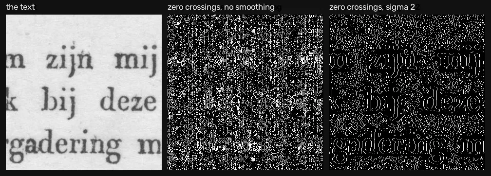
A crop of printed text, its zero-crossings with no smoothing which fill the paper with speckle, and its zero-crossings after smoothing which follow the letters — The text, its zero-crossings raw, and after smoothing. Without smoothing the blank paper is full of crossings; the paper has not changed, only what we were willing to call a sign change. Source: “Departementaal Dagblad van de Zuiderzee, 1814” (Rijksmuseum, Wikimedia Commons), CC0.

What it means: unsmoothed, 96.3% of the zero-crossings are not edges. They are the scan’s grain crossing zero, and the Laplacian cannot tell the difference because a sign change carries no notion of size. Smoothing to σ = 4 removes three quarters of them — and notice what it does not do: the share that are real only climbs from 3.7% to 6.0%. Smoothing suppresses the noise and the text together.

This is the whole argument for the LoG being a scale choice rather than a cleanup, and for Canny being built on the first derivative, where a threshold on magnitude can throw away a weak crossing that a sign test is blind to.

Where this breaks

Zero-crossings have two properties that no threshold can repair.

Every crossing weighs the same. The sign of $\nabla^2 I$ flips across a faint faint shadow on the base as it does across a column silhouette. Lesson 2’s magnitude told you how strong an edge was; a crossing tells you only that one is there. Ranking edges, which is what the next lesson depends on, is not available from this operator alone.

Smoothing controls the damage, and it costs structure. Measured on the canonical frame, adding noise of sigma 10 and counting zero-crossing pixels against the clean image:

Gaussian sigma	crossing px, clean	crossing px, noisy	ratio	closed contours, clean
1.0	25,625	70,776	2.76x	0.334
1.4	19,444	37,347	1.92x	0.277
2.0	13,621	15,525	1.14x	0.243
3.0	8,161	8,320	1.02x	0.156

At sigma 1.0 noise nearly triples the structure. At sigma 3.0 it adds 2%, and the clean image is down to 8,161 crossing pixels from 25,625. A third of the detail went with the noise.

The last column is the one that contradicts the usual claim. Zero-crossings of a continuous Laplacian of Gaussian form closed contours, and that survives discretization on synthetic input: a rendered disc gives a closed fraction of 1.000 at every sigma tested. On a photograph it does not. Only 33.4% of the crossing components are closed at sigma 1.0, falling to 15.6% at sigma 3.0, since real contours run off the frame, meet at junctions, and get cut where the response is too flat to count. Closure is a property of the ideal operator, not of the edge map you actually get.

So the first derivative gives strength and thickness, and the second gives position and no strength. Canny’s answer was not to choose. He kept the gradient and added two mechanisms: one that fixes the width without touching the threshold, and one that fixes the coverage without touching the width [2] [3]. Lesson 4 takes them apart.

References

[1] Marr, D., & Hildreth, E. (1980). Theory of edge detection. Proceedings of the Royal Society of London B, 207(1167), 187-217. doi:10.1098/rspb.1980.0020

[2] Canny, J. F. (1986). A Computational Approach to Edge Detection. IEEE Transactions on Pattern Analysis and Machine Intelligence, 8(6), 679-698. doi:10.1109/TPAMI.1986.4767851

[3] Gonzalez, R. C., & Woods, R. E. (2018). Digital Image Processing (4th ed.), section 10.2 “Point, Line, and Edge Detection”, The Marr-Hildreth Edge Detector, p. 786. Pearson.

[4] Lowe, D. G. (2004). Distinctive Image Features from Scale-Invariant Keypoints. International Journal of Computer Vision, 60(2), 91-110. doi:10.1023/B:VISI.0000029664.99615.94

Tagged