Image Sensing: What the Number in a Pixel Actually Counts

What the number in a pixel actually counts, and how far you can trust it.

That is the unit. Five lessons: how light becomes an integer, why that integer is a random variable, what the camera did to it before you ever saw the file, how a stack of exposures turns back into light with a physical unit attached, and where the colour of that light comes from when every photosite can only measure one.

Before this

Nothing, beyond having seen an image as an array of numbers. This unit sits at the bottom of the track: it starts at the photosite and stops before anything is done to the result. What happens next — the grid those counts sit on, how finely they are written down, and the coordinate systems the colour goes into — is The Image as Data.

The scene everything is measured on

Every number in this unit comes from one photograph, or rather from eighteen photographs of one scene: “Luxo Double Checker” from Mark Fairchild’s HDR Photographic Survey [2]. A desk lamp with the bulb lit, a GretagMacbeth ColorChecker on the right under direct light, a second identical chart on the left with no direct light at all, a small plastic cow, and a dark table running out of the frame.

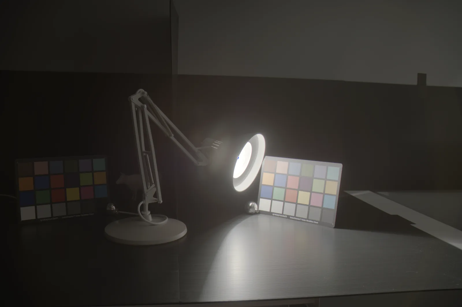
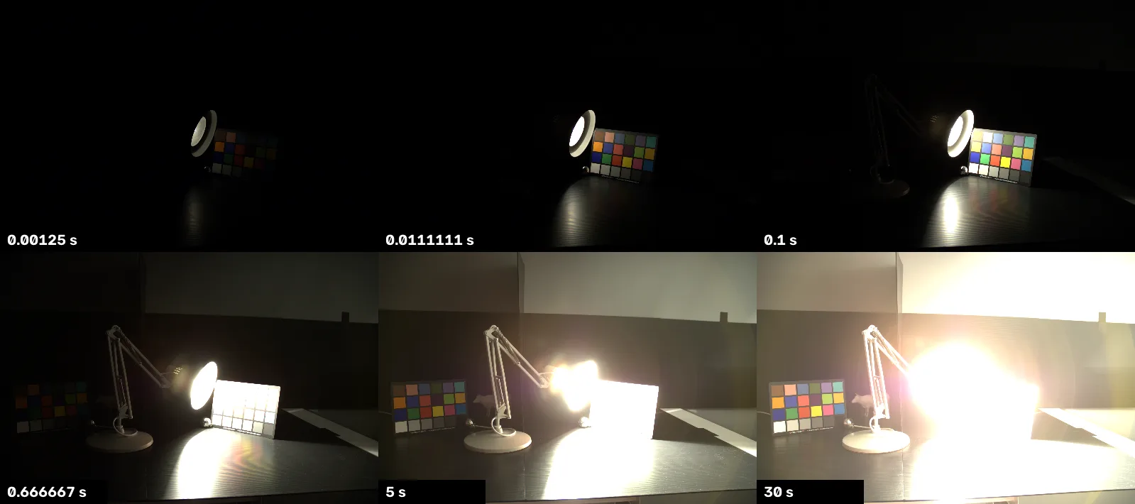
Fairchild built the scene to characterise a camera, which is the same job this unit does on the page. Three things about it are why every lesson can be checked rather than asserted:

• Eighteen exposures, a stop apart, from 1/800 s to 30 s, all at ISO 100 on a Nikon D2x. The last three are all 30 s, because the camera ran out of shutter.
• Fifty-four points metered in the room with a Konica Minolta CS-100 colorimeter at a 1° angle, from 0.015 to 2530 cd/m². That is a measured range of 17.4 stops, and it is ground truth that never passed through any of our code.
• Forty-eight uniform patches, twenty-four on each chart, of known relative reflectance. The bottom row of each is a neutral ramp, white through black, and three of the five lessons work on it.

The two charts are the same object under lighting 9 stops apart. That single fact is what makes the unit’s arguments visible instead of algebraic.

Topics

1. From photons to counts. A photosite collects electrons and a converter turns them into an integer. What sets the floor, what sets the ceiling, why the same count can mean two different amounts of light [1], and what the CMOS sensor under all of it actually is [5].
2. Sensor noise and dynamic range. Read the same photosite twice and you get two numbers. The variance of a count against its mean is a straight line whose slope is the sensor’s gain, and that line is how full well, read noise and dynamic range are measured rather than looked up [4][6].
3. The camera response curve. Raw is proportional to light. The file you opened is not. What the tone curve did, how to see it, and which algorithms it quietly breaks [3][7].
4. High dynamic range imaging. No single exposure holds this scene. Merge the bracket into one radiance map, fit a single scale factor on one patch, and check the rest against the colorimeter [3][8].
5. Sensing colour: the Bayer mosaic. Silicon is colourblind, so a mosaic of filters gives each photosite one channel and an algorithm invents the other two. Two thirds of every colour image is that invention, and it costs twenty-eight times more at an edge than on a flat patch.

The order is a ramp. Lesson 1 says what a count is under ideal conditions, lesson 2 is where that idealisation breaks, lesson 3 is what the camera does about it for your eyes, and lesson 4 is the representation that undoes all of it and gets back to light. Lesson 5 is the one property of the count this unit had left aside: which wavelengths it counted.

How they fit together

What the unit measures

Every number below comes from output/sensing_numbers.json, computed from the eighteen raw files by uv run sensing-experiments.

Result	Measurement
A count is proportional to exposure, until it is not	The lit chart’s white patch reads 109 → 226 → 460 → 961 → 1902 DN as the shutter doubles, then stays within a digital number or two of 3875 DN for the last twelve exposures
The sensor’s ceiling is not the file’s ceiling	LibRaw reports a white level of 4095 DN; the green channels stop at 3880, red and blue at 4095, and the file’s own camera tag says 3827
Gain, from the slope of variance against signal	0.294 ± 0.007 DN per electron on the green channel, $R^2 = 0.986$ over 27 signal levels — 3.40 electrons per DN
Full well and dynamic range	13,199 e⁻, and at least 11.21 stops between saturation and the dark-frame noise floor of 1.64 DN (5.6 e⁻)
The developed file is not proportional to light	Over the neutral ramp, the code values sit a mean of 9.6 code values away from the sRGB curve, and no single exponent fits them ($\gamma = 1.47$, $R^2 = 0.987$, and wrong at both ends)
A merged bracket can be checked against an instrument	One scale factor fitted on one patch; the other 47 land a median of 0.198 stops from the colorimeter, 0.109 stops across the twelve neutral patches

The last row is the one worth arguing about, and lesson 4 argues about it: the failures are all at the dark end, where flare from the bulb and the noise floor both live.

Reproducibility

Parameter	Value
CPU	12th Gen Intel Core i7-12700H, 20 threads
GPU	none used; every measurement here runs on the CPU
RAM / OS	31 GB · Ubuntu 22.04.5 LTS, kernel 6.8.0-136
Key versions	Python 3.12.9, NumPy 2.5.2, OpenCV 5.0.0, rawpy 0.27.0 on LibRaw 0.22.1 [10]
Camera	Nikon D2x, f/3.5, 18 mm, ISO 100, 18 exposures from 1/800 s to 30 s, 20 April 2006
Data	HDRPS “Luxo Double Checker” [2]: 18 NEF files fetched from the survey’s RAW archive, plus its measurement table. 54 metered points, Konica Minolta CS-100, 1° angle
Commands	uv sync --extra sensing, then uv run sensing-download and uv run sensing-experiments; the photographs come from uv run data-experiments
In the wild	Four Wikimedia Commons files — a long-exposure astrophotograph, a ColorChecker, a twilight landscape and a street scene, all CC0, public domain or CC BY 4.0. Registered in CondadosAI/cv-assets with verified licences and a sha256 each; downloaded, never redistributed
Runs	one; every statistic pools thousands of pixels, and the three 30 s frames are the repeats
Excluded	no timing is reported in this unit — every number is a count, a ratio or a fitted coefficient

The lessons carry no reproducibility table of their own — this one covers all five, which is how unit 3.1 has always worked and how the whole track now works.

Every lesson also repeats its measurement on a photograph. A long-exposure frame of the Orion Nebula has a background whose noise is as large as its signal, 1421 clipped star cores and 12,641 pixels crushed to zero; a photographed ColorChecker shows that reading a JPEG as if it were linear understates the range between white and black by 10.5×; a twilight landscape clips 31 pixels in 33.6 million and needed no bracket at all; and a street scene puts 5.4× more red-blue disagreement on its edges than on its flat areas.

Limitations & caveats

• One sensor, from 2004. Gain, full well, read noise and the tone curve are properties of this camera, not of cameras. Shot noise is physics and generalises; none of the rest does. A modern phone sensor has a smaller well, a lower read noise, and a tone curve nothing like this one.
• ISO is fixed at 100 across the bracket, so nothing here measures what gain does. Lesson 2 states the relationship and says plainly that it did not measure it.
• Read noise is bounded, not measured. The repeated frames are 30 s long, so the darkest signal they contain is a few hundred DN; the transfer curve’s intercept is an extrapolation and comes out negative. The 1.64 DN figure is the spatial spread of a dark corner of the shortest exposure, which includes fixed pattern and dark current, so it is an upper bound and the dynamic range built on it is a lower one.
• The metered points are 1° spots, and our patches are rectangles. They cover the same paint but not the same solid angle, and the alignment between the survey’s map and the raw frame was recovered by us, not published by them. The check on that alignment is a rank correlation of 0.982 on the lit chart and 0.955 on the shadowed one, which is enough to rule out a mislabelled lattice and not enough to call it exact.
• Colour is borrowed. Lesson 4 converts camera channels to luminance with the matrix row Fairchild fitted for this camera, on this scene. It is the one number in the unit we did not measure ourselves.

Where this lands

Nothing on the site runs this on hardware yet. A unit closes on a measured system when one exists, and here one does not: say that rather than invent it. The natural candidate is a detector fed with real high-ISO frames instead of clean ones, which would put lesson 2’s noise model in front of something that has a score. If that gets written, it will be linked from here.

What the unit does hand forward is the linearity claim. Every method that assumes brightness is proportional to light — photometric stereo, shape from shading, brightness constancy in optical flow — is relying on lesson 1 and being warned by lesson 3.

Further reading

• Go deeper: Gonzalez & Woods, Digital Image Processing (4th ed.), §2.3 “Image Sensing and Acquisition” [1] — the textbook treatment of the same pipeline, from a single sensing element to the array.
• The wider map: Szeliski, ch. 2 “Image formation” [9], for where the sensor sits relative to the optics in front of it and the processing after it.
• The standard practitioners use: EMVA Standard 1288, Release 4.0 Linear [6]. It specifies how gain, read noise and dynamic range are to be measured on an industrial camera, and it is what our informal version approximates.
• Related on CondadosAI: the image as data is the unit above this one · 2D convolution is where the array gets processed · edge detection is what happens to it next.

References

[1] Gonzalez, R. C., & Woods, R. E. (2018). Digital Image Processing (4th ed.), ch. 2 “Digital Image Fundamentals”, §2.3 “Image Sensing and Acquisition”, p. 41, and §2.4 “Image Sampling and Quantization”, p. 47. Pearson.

[2] Fairchild, M. D. (2007). The HDR Photographic Survey. Proceedings of the IS&T 15th Color and Imaging Conference, pp. 233–238. doi:10.2352/CIC.2007.15.1.art00044 — the scene, its 54 metered points and its raw exposures: markfairchild.org/HDR.html. Used here for research and non-commercial publication, as the survey’s terms require; images are downloaded, never redistributed.

[3] Debevec, P. E., & Malik, J. (1997). Recovering high dynamic range radiance maps from photographs. SIGGRAPH ‘97, pp. 369–378. doi:10.1145/258734.258884

[4] Healey, G. E., & Kondepudy, R. (1994). Radiometric CCD camera calibration and noise estimation. IEEE Transactions on Pattern Analysis and Machine Intelligence, 16(3), 267–276. doi:10.1109/34.276126

[5] Fossum, E. R. (1997). CMOS image sensors: electronic camera-on-a-chip. IEEE Transactions on Electron Devices, 44(10), 1689–1698. doi:10.1109/16.628824

[6] European Machine Vision Association (2021). EMVA Standard 1288, Release 4.0 Linear: Standard for Characterization of Image Sensors and Cameras, effective 21 June 2021. emva.org

[7] Mitsunaga, T., & Nayar, S. K. (1999). Radiometric self calibration. CVPR 1999, pp. 374–380. doi:10.1109/CVPR.1999.786966

[8] Hasinoff, S. W., Sharlet, D., Geiss, R., Adams, A., Barron, J. T., Kainz, F., Chen, J., & Levoy, M. (2016). Burst photography for high dynamic range and low-light imaging on mobile cameras. ACM Transactions on Graphics, 35(6), 1–12. doi:10.1145/2980179.2980254

[9] Szeliski, R. (2022). Computer Vision: Algorithms and Applications (2nd ed.), ch. 2 “Image formation”. Springer. Free PDF

[10] LibRaw (0.22.1) and rawpy (0.27.0). Raw image decoding. libraw.org/docs · rawpy documentation