
Before this unit: Homogeneous coordinates
How to Compute a Homography from Four Points
Lesson 3 of Image Alignment. Each point pair gives two linear equations in the nine entries of H, and the answer is the singular vector of the smallest singular value. Normalising the coordinates drops the condition number from 53,466 to 6.4, and on this court changes the answer by under 0.2 cm. What decides the error is where the pixels are: one pixel is 0.6 cm of court at the near baseline and 8.1 cm at the far one.
Show the computer four points you can see in both pictures, say the four corners of a court, and it can work out the whole homography. Each pair of points gives two equations, four pairs give the eight the homography needs, and one standard piece of linear algebra solves them.
Where people compute one:
- Sports analytics. Click four court or pitch corners in a frame and every player position can be read in metres. The lab below lets you do that on a real frame.

- Camera calibration. Zhang’s method, the one behind chessboard calibration in OpenCV, starts from a homography between the board and each photograph [6].
- Security cameras and floor plans. Four points on the floor matched to a building plan map every person the camera sees onto the plan.
- Augmented reality on a flat marker. The printed square in the camera view gives four corners, and the homography places the graphics on it.
A homography has nine entries and one of them is redundant, so it takes eight equations to fix. Each point pair supplies two, both linear in those nine entries. Stack them into a matrix and the homography is the direction sends to zero, read off the last singular vector of an SVD. On this court the fit agrees with OpenCV to 0.00026 mm. Normalising the coordinates first drops the condition number of from 53,466 to 6.4, and changes the answer here by under 0.2 cm. What does decide the error is where each pixel sits: one pixel is 0.6 cm of court at the near baseline and 8.1 cm at the far one.
Where we are
Part of image alignment.
Lesson 2 showed that a 3×3 with eight free
numbers is the right model for a plane seen by a camera, and that four corners of the
court fix it well enough to land a held-out corner 0.47 cm from the rulebook. It used
getPerspectiveTransform as a black box. This lesson opens it, and then asks what the
box does with more than four points and with points that are slightly wrong.
Two equations per point
A pair says that sends to something proportional to . Write the rows of as , , . “Proportional” means
Multiply out the denominators and both equations become linear in the nine unknowns:
Each pair becomes two rows of a matrix , and with the nine entries of laid out in a column [1]. This is the Direct Linear Transform. With four pairs is 8×9, so exactly one direction is sent to zero. With more pairs and a little noise nothing is sent exactly to zero, and the best answer is the unit vector shrinks the most. In both cases that vector is the right singular vector of the smallest singular value.
The whole method in code, written out and checked against OpenCV:
import cv2
import numpy as np

def dlt(src, dst):
    """Homography with dst ~ H @ src, from four or more (N, 2) point pairs."""
    rows = []
    for (x, y), (u, v) in zip(src, dst):
        rows.append([-x, -y, -1, 0, 0, 0, u * x, u * y, u])
        rows.append([0, 0, 0, -x, -y, -1, v * x, v * y, v])
    _, _, vt = np.linalg.svd(np.asarray(rows))
    H = vt[-1].reshape(3, 3)             # the direction A shrinks the most
    return H / H[2, 2]

image = np.array([[-18.52, 587.39], [987.25, 959.91], [669.68, 500.09], [1555.24, 663.22]])
court = np.array([[0.0254, 0.0254], [0.0254, 6.0746], [4.6004, 0.0254], [4.6004, 6.0746]])
H_img2court = dlt(image, court)
print(np.abs(H_img2court - cv2.getPerspectiveTransform(image.astype(np.float32),
                                                       court.astype(np.float32))).max())
#include <opencv2/core.hpp>
#include <opencv2/imgproc.hpp>
#include <iostream>
cv::Mat dlt(const std::vector<cv::Point2d>& src, const std::vector<cv::Point2d>& dst) {
cv::Mat A((int)src.size() * 2, 9, CV_64F);
for (size_t i = 0; i < src.size(); ++i) {
double x = src[i].x, y = src[i].y, u = dst[i].x, v = dst[i].y;
double r1[9] = {-x, -y, -1, 0, 0, 0, u * x, u * y, u};
double r2[9] = {0, 0, 0, -x, -y, -1, v * x, v * y, v};
for (int j = 0; j < 9; ++j) { A.at<double>(2 * i, j) = r1[j]; A.at<double>(2 * i + 1, j) = r2[j]; }
}
cv::Mat w, u, vt;
cv::SVD::compute(A, w, u, vt, cv::SVD::FULL_UV);
cv::Mat H = vt.row(8).reshape(1, 3);
return H / H.at<double>(2, 2);
}What normalising changes, measured
Six pairs this time: the four corners plus the two ends of the near centre line, each given 1 px of random noise, 1,000 times. The quantity scored is the error at the far baseline, the part of the court the fit never saw.
| six noisy pairs | median | 95th percentile |
|---|---|---|
| raw coordinates | 31.03 cm | 53.83 cm |
| normalised | 31.09 cm | 53.91 cm |
The largest difference in any single trial is 0.20 cm. Mapping pixel to pixel instead, image to a bird’s-eye view, the raw condition number reaches 9.2 million and the normalised one is 6.3. Hartley’s paper is about a case where the difference is large, the eight-point estimate of the fundamental matrix [2], the two-view problem behind structure from motion. On a homography from a handful of well-spread points in double precision, it is small.
What normalising guarantees is that the answer does not depend on where you put the origin. Shift every pixel coordinate by the same amount, solve, and shift back:
| origin moved by | 0 | 1,000 px | 10,000 px | 100,000 px |
|---|---|---|---|---|
| normalised, far baseline error | 29.073 cm | 29.073 cm | 29.073 cm | 29.073 cm |
| raw, far baseline error | 28.925 cm | 28.975 cm | 28.993 cm | 28.995 cm |
The raw answer depends on a choice that has nothing to do with the court. Hartley and Zisserman make that the argument for normalising [1]: it costs two 3×3 multiplications and removes a dependence that should never have been there. Do not expect it to rescue a bad fit.
Where the error goes
The same pixel error means very different things across this court. At the near right corner, one pixel of image is 0.26 × 0.61 cm of court (along the image’s and ); at the near kitchen line’s centre, 0.61 × 3.09 cm; at the far right corner, 1.08 × 8.08 cm. The far baseline error of 38.4 cm from four points is under 5 px, and the noise study puts 1 px of noise on each corner and gets a median of 38.5 cm there from four points: the far court is where any pixel error is magnified.
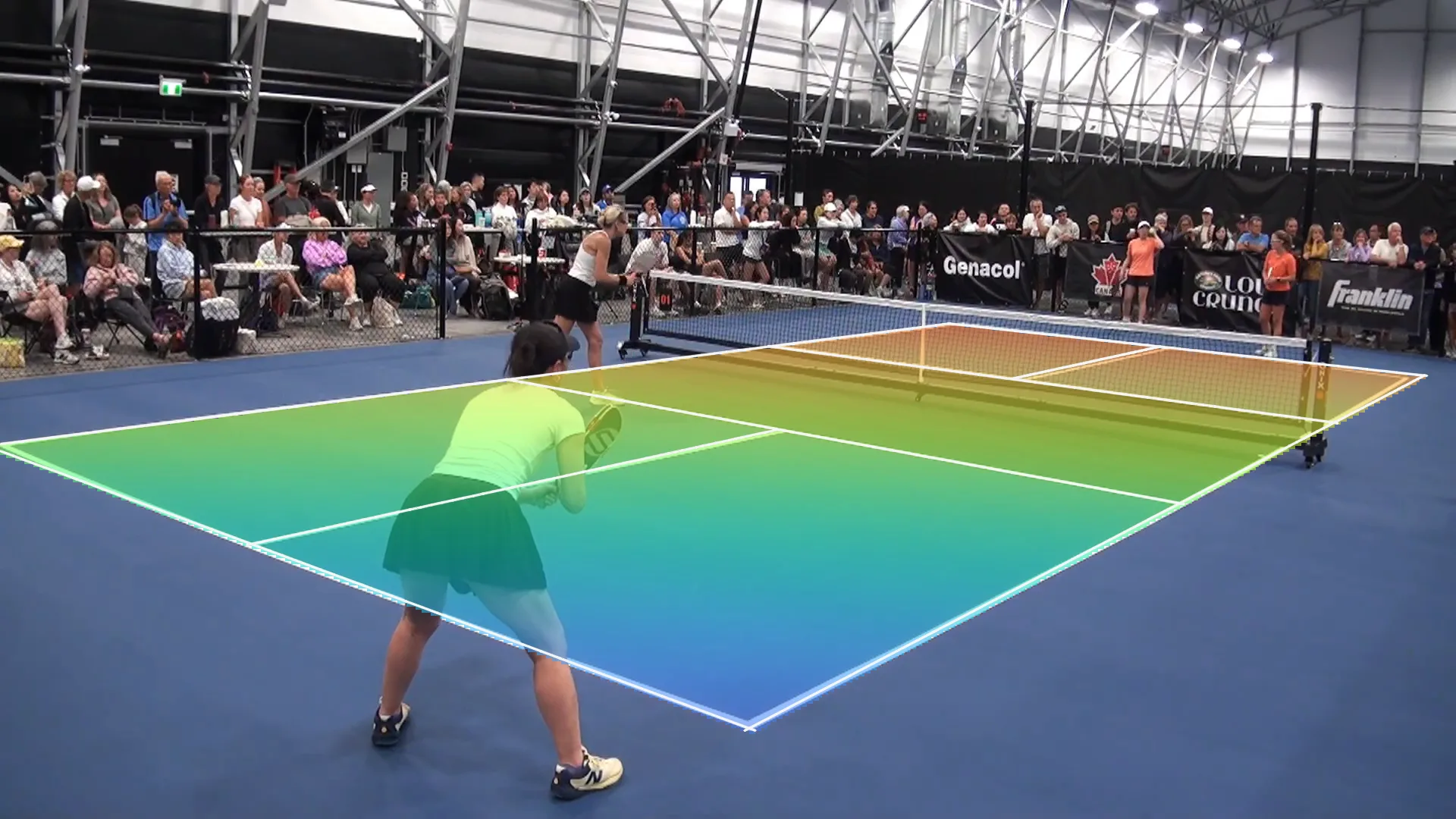
Adding the two centre-line corners improves everything near them (NKC from 5.63 to 3.18 cm, the far baseline from 38.4 to 31.7) and makes the far sideline worse, 5.95 to 8.53 cm. More points near the camera are not what the back of the court needs; points at the back are, and on this frame the net hides them.
Now you try
Build the system yourself. Click a point on the court diagram (A), then the same point on the photograph (B). From four pairs on, the lab solves the DLT above in your browser, normalised, and draws every line of the court pushed from A into B. With exactly four pairs the residual is zero whatever you clicked; add a fifth and it becomes a measurement. Click one pair deliberately wrong and watch the whole court bend towards it.
Frame 45000 of "2026.07.25 WD Open … (Gold Medal match)" by pickleball4you, CC BY 3.0.
The second lab shows the same fit from the inside. The DLT tab shows ‘s singular values live. Drag a corner and watch stay at zero while the others move: four pairs always have an exact solution. Toggle Normalise and watch jump from thousands to single digits while the court overlay does not move.
Frame 45000 of "2026.07.25 WD Open … (Gold Medal match)" by pickleball4you, CC BY 3.0.
In the wild
On the outdoor court [5], where the camera is closer and the near half fills the frame, one pixel is 0.31 × 0.89 cm of court at the centre-line corner of the baseline and 0.64 × 3.51 cm at the right end of the kitchen line. The homography through four corners lands NBC 0.77 cm out and the kitchen-line corner NKC 11.3 cm out. One pixel at NKC is 0.53 × 2.33 cm, so that is about five pixels. That is the same story as indoors, a few pixels of disagreement turned into centimetres by where they happen, and one of the four corners this fit used is 140 px outside the frame, so its position is an extrapolation of two fitted lines.
Where this breaks
The DLT believes every pair it is given. Give it the six pairs again, but with one mislabelled: the pixel of the near-right kitchen corner handed in as the centre-line corner beside it, the kind of mistake a matcher makes when two corners look alike, and the one Lowe’s ratio test catches only some of the time.
| held-out check | six correct pairs | one pair mislabelled |
|---|---|---|
| NBC | 0.25 cm | 5.69 cm |
| near centre line | 2.13 cm | 47.9 cm |
| far right sideline | 8.53 cm | 449 cm |
| far baseline | 31.7 cm | 1,757 cm |
One wrong pair out of six puts the far baseline 17.6 m out. Least squares averages, and an average has no way to tell one bad value from five good ones. A smaller slip, the right corner found 25 px off along its line, costs less (54 cm at the far baseline) and is as undetectable from the fit itself.
Next
The fix is not a better average. It is to fit many times on minimal sets of four and keep the fit most of the pairs agree with, which is RANSAC, lesson 4 of this unit [3]. Szeliski puts it in the same section as the least-squares fit for this reason [4].
Run it: every code block on this page has a cell in the unit’s notebook, open it in Colab.
References
[1] Hartley, R., & Zisserman, A. (2004). Multiple View Geometry in Computer Vision (2nd ed.), §4.1 “The Direct Linear Transformation (DLT) algorithm”, p. 88, and §4.4 “Transformation invariance and normalization”, p. 104. Cambridge University Press.
[2] Hartley, R. I. (1997). In Defense of the Eight-Point Algorithm. IEEE Transactions on Pattern Analysis and Machine Intelligence, 19(6), 580–593. doi:10.1109/34.601246
[3] Hartley, R., & Zisserman, A. (2004). Multiple View Geometry in Computer Vision (2nd ed.), §4.7 “Robust estimation”, p. 116, and §4.8 “Automatic computation of a homography”, p. 123. Cambridge University Press.
[4] Szeliski, R. (2022). Computer Vision: Algorithms and Applications (2nd ed.), §8.1.1 “2D alignment using least squares” and §8.1.4 “Robust least squares and RANSAC”. Springer. Free PDF
[5] pickleball4you (2024). 2024.08.30 MS4.0 Philip Wong vs Tristan Clark (Round Robin, match 6). YouTube, CC BY 3.0. youtube.com/watch?v=K0qrASvix3Y
[6] Zhang, Z. (2000). A Flexible New Technique for Camera Calibration. IEEE Transactions on Pattern Analysis and Machine Intelligence, 22(11), 1330–1334, §2.2 “Homography between the model plane and its image” in the technical report MSR-TR-98-71. doi:10.1109/34.888718