What Is a Homography?

A homography is the rule that moves every point of a flat surface from one photograph to where the same point appears in another photograph of that surface. Photograph a court, a page or a wall from any angle, find four points you can recognise in both views, and the homography tells you where every other point goes.

Once you know what to look for, homographies are everywhere a camera looks at something flat:

• Sports graphics. The radar view of a broadcast, the player positions in the animation above, and the distances a stats overlay quotes are all image points mapped onto the playing surface.
• Graphics painted onto the ground. An advert or a line that appears to lie on the pitch is an image warped onto the pitch’s plane and drawn under the players:

• Document scanners. A phone app that flattens a page photographed at an angle finds its four corners and moves them to a rectangle with one homography:

• Panoramas. Photographs taken from one spot while turning the camera are related by homographies, which is how panorama modes join them [12]:

• Camera calibration. The standard method photographs a flat chessboard several times and starts from the homography between the board and each photo [11].
• And in parking cameras that stitch a top-down view of the car’s surroundings, in projectors that correct a tilted image, and in aerial photos aligned to a map.

The rest of this page, and the five lessons under it, build that rule from the ground up on one real photograph, and measure how well it works.

Taking a photograph of a flat thing and working out, for every pixel, where on that thing it lies.

That is the whole unit. Five lessons: what a 2×2 matrix does to a picture and the one thing it can never do, the 3×3 that does it, how four point pairs determine that 3×3, how to find it when some pairs are wrong, and how to resample an image through it once you have it. Gonzalez and Woods file the same problem under geometric transformations and image registration [7].

Before this

You need homogeneous coordinates. Every map in this unit is a matrix acting on $(x, y, 1)$, and the lesson that explains why also measures the vanishing point this unit keeps returning to. Correspondences come from SIFT in a panorama and from painted lines here; the edge detection unit is where finding those lines starts.

The frame everything is measured on

One frame of the 2026 WD Open women’s doubles gold-medal match, filmed by a fixed camera standing behind the near-left corner of the court [9]. Frame 45000, 1920×1080, which is 1,501.5 s into the match.

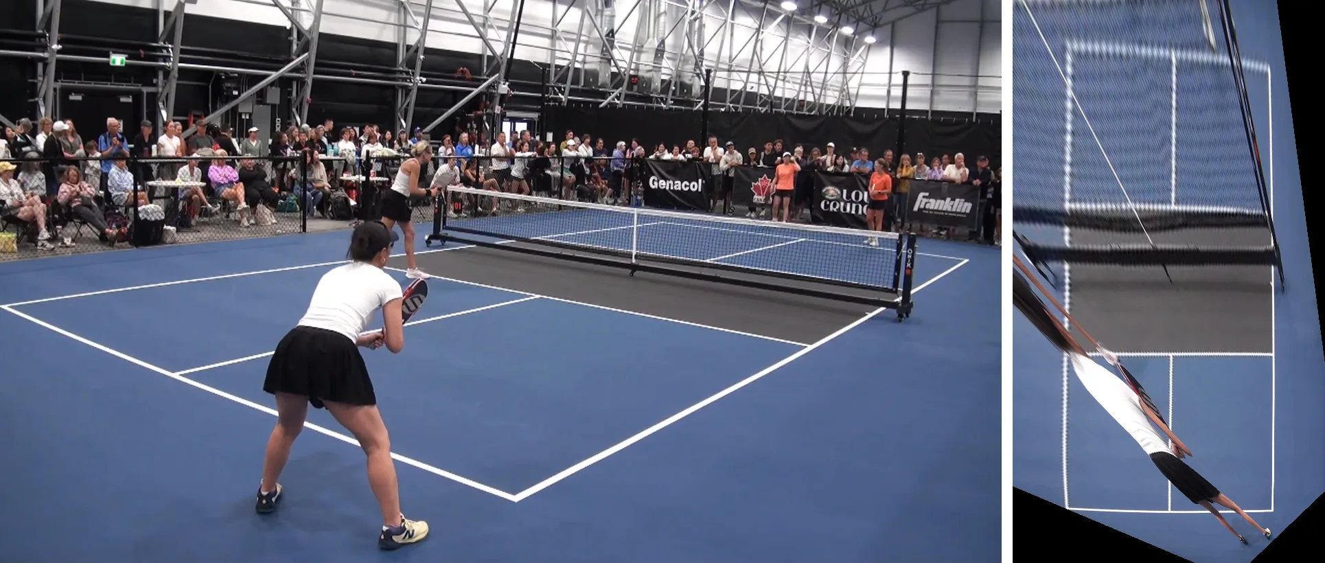
A court is the best possible object for this unit because its size is written down. The USA Pickleball rulebook fixes it at 13.41 × 6.10 m with the non-volley lines 2.13 m from the net, measured to the outside edge of 5.08 cm lines [8], so every claim below is a distance in centimetres against a published dimension rather than an alignment that looks right.

Twelve points on it have names: where each painted line crosses another. Four of them, the corners of the near half, define the fit in every lesson. A fit through four points reproduces those four exactly, so their error is zero and proves nothing. Everything else is the evidence:

Held-out check	What it must equal
NBC, NKC: where the near centre line meets the baseline and the kitchen line	their court positions
the near centre line, along its whole length	$y = 3.05$ m
the right sideline beyond the net	$y = 6.07$ m
the far baseline, where it shows right of the net post	$x = 13.38$ m

Try the whole unit in one move

Pick a point on the court diagram, then the same point on the photograph, four times. The browser solves for the homography on the spot and draws the whole court from the diagram onto the photo. Every lesson below explains one part of what happened.

Topics

1. What a 2×2 matrix does to a picture. Four numbers move the whole plane: where do they send it, what does the determinant measure, and what is the one thing no 2×2 can do to a court?
2. Affine and projective: the 3×3. One extra coordinate buys translation, and one extra row buys perspective [2]. How much does each buy on a real court?
3. Computing a homography: the DLT. Four point pairs give eight equations in nine unknowns [1]. How is the answer read off, what does normalising the coordinates change [6], and where does the error go?
4. RANSAC. The DLT trusts every pair it is given. How do you fit a model when a third of the pairs are wrong [5]?
5. Warping and blending. With the map in hand, how do you move the pixels through it without leaving holes, and how do you combine several frames into one?

The order is the ramp: lesson 1 is the criterion (parallel lines on the court are not parallel in the photo), lesson 2 is the simplest map that meets it, lesson 3 computes it and shows where it fails, lesson 4 repairs that failure, and lesson 5 puts the result to use.

How they fit together

What the unit measures

Every lesson carries its own numbers. The ones that decide the order the lessons are in, all from output/alignment_numbers.json, all in centimetres on the court and all on paint the fit never saw:

	NBC	NKC	near centre line	far right sideline	far baseline
affine through 3 corners	91.6	188.5	125.6	397.0	308.8
affine, least squares on 4	122.4	34.1	78.6	105.1	551.6
homography through 4	0.47	5.63	2.66	5.95	38.4
homography, least squares on 6	0.25	3.18	2.13	8.53	31.7
homography through 4, lens corrected	0.51	5.42	2.74	1.96	24.1

Two things in that table set up the unit. The step from affine to projective cuts the error by 8× at the far baseline and by up to 195× at NBC, which is lesson 2. And the homography’s worst number, 38 cm at the far baseline, is not a failure of the model: one pixel there spans 8.1 cm of court, against 0.6 cm at the near baseline, so the far baseline’s 38.4 cm is under 5 px. Lesson 3 is about where error goes.

Reproducibility

Parameter	Value
CPU	12th Gen Intel Core i7-12700H, 20 threads
GPU	none used; everything runs on the CPU (the machine has an RTX 3060 Laptop GPU)
RAM / OS	31 GB · Ubuntu 22.04.5 LTS, kernel 6.8.0-138
Key versions	Python 3.12.9, OpenCV 5.0.0 [10], NumPy 2.5.2
Data	YouTube T5rmWjvt8Os by pickleball4you, CC BY 3.0 [9]: frame 45000 (shown) and the per-pixel median of 31 frames, 44100 to 45900 every 60 (measured)
In the wild	YouTube K0qrASvix3Y by pickleball4you, CC BY 3.0, 450–520 s, 31 frames every 60, median (lessons 1–3 and 4.1-L1); BarcelonaHarbour1.jpg and BarcelonaHarbour2.jpg by Pap3rinik, Wikimedia Commons, public domain, resized to 1600 px (lesson 5). All registered in CondadosAI/cv-assets with licence and sha256, downloaded, never redistributed
Court model	USA Pickleball 2026 rulebook, Rule 3.A [8]; lines at their centres, 2.54 cm inside each nominal dimension
Commands	uv run align-download, then uv run align-experiments and uv run align-figures
Runs	deterministic, except the DLT noise study: 1,000 draws of σ = 1 px from seed 20260926
Excluded	no timing is reported in this unit; every number is a distance, a count or a ratio

Every number in the posts is a key in output/alignment_numbers.json. The frame and the median plate are served from this site as lossless WebP, so the notebook measures the same pixels the repository does. The 31 frames are served at 960 px for the notebook’s median demonstration; align-download --from-youtube fetches them at full resolution.

Why the median. The camera never moves in that minute, and the players do. In frame 45000 the near player’s white shirt stands on the left sideline, and a detector looking for white paint takes it for paint. The median of 31 frames is the court with nobody on it; the six near-court corners found on it and on frame 45000 agree to within 1.3 px.

Limitations & caveats

• One camera, one court, one minute. Everything is measured on a single fixed view. The ordering (affine far worse than projective) is geometry and will hold anywhere; the centimetre values belong to this lens, this distance and this angle.
• The far half of the court is mostly not evidence. Seen through the net’s mesh, a painted line turns into a dotted band as wide as the strip searched around it, and a line fitted to a uniform band returns the middle of the strip, which is the prediction it started from. The net region is excluded by a polygon drawn by hand, and the far half contributes only the two stretches of paint that show clear of it.
• The lens is not a pinhole. The near baseline bows by 7.7 px across the frame. A one-parameter division model fitted to the near lines straightens it to 0.16 px and cuts the far-sideline error from 5.95 to 1.96 cm. Its centre is assumed to be the frame centre, and no calibration of this camera exists to check that. The lessons work in raw pixels; the corrected row above is the size of what they leave on the table. The distortion lesson covers the model.
• Paint was found as a ridge, and that choice moves the numbers. A brightness threshold alone also admits the pale grey of the non-volley zone. With it, the far baseline error is 81.3 cm instead of 38.4, because the grey sits on one side of the kitchen line and drags its fit.
• The outdoor clip reproduces to the frame, not to the byte. yt-dlp --download-sections re-encodes the cut with the local encoder, so the section file’s hash differs between machines. The outdoor numbers are tied to frame indices within the section, not to a checksum.
• The seed does not leak, and that was checked. The lines are found near four corner positions typed in by eye. Moving those by up to 5 px in 20 random trials moves no fitted corner by more than 0.58 px.

Where this lands

The measured system this unit points at does not exist as a post yet: a ball and player tracker that puts every bounce on the court in metres runs on this homography, and the article on it is pending. Until then the nearest thing on the site is structure from motion, which is what you need when the scene is not a plane and one 3×3 no longer describes it.

Further reading

• Go deeper: Hartley & Zisserman, ch. 4 “Estimation – 2D Projective Transformations” [1], for the DLT, the cost functions it approximates and the normalisation argument in full.
• The practitioner’s map: Szeliski, ch. 8 “Image Alignment and Stitching” [3], and his earlier tutorial of the same name [4], for how panorama software strings these steps together.
• Related on CondadosAI: homogeneous coordinates is the prerequisite · camera models and PnP is the 3-D version of the same fit.

References

[1] Hartley, R., & Zisserman, A. (2004). Multiple View Geometry in Computer Vision (2nd ed.), ch. 4 “Estimation – 2D Projective Transformations”, §4.1 “The Direct Linear Transformation (DLT) algorithm”, p. 88, and §4.4 “Transformation invariance and normalization”, p. 104. Cambridge University Press.

[2] Hartley, R., & Zisserman, A. (2004). Multiple View Geometry in Computer Vision (2nd ed.), §2.4 “A hierarchy of transformations”, p. 37. Cambridge University Press.

[3] Szeliski, R. (2022). Computer Vision: Algorithms and Applications (2nd ed.), ch. 8 “Image Alignment and Stitching”, §8.1 “Pairwise alignment” and §8.4 “Compositing”. Springer. Free PDF

[4] Szeliski, R. (2006). Image Alignment and Stitching: A Tutorial. Foundations and Trends in Computer Graphics and Vision, 2(1), 1–104. doi:10.1561/0600000009

[5] Fischler, M. A., & Bolles, R. C. (1981). Random Sample Consensus: A Paradigm for Model Fitting with Applications to Image Analysis and Automated Cartography. Communications of the ACM, 24(6), 381–395. doi:10.1145/358669.358692

[6] Hartley, R. I. (1997). In Defense of the Eight-Point Algorithm. IEEE Transactions on Pattern Analysis and Machine Intelligence, 19(6), 580–593. doi:10.1109/34.601246

[7] Gonzalez, R. C., & Woods, R. E. (2018). Digital Image Processing (4th ed.), §2.6 “Introduction to the Basic Mathematical Tools Used in Digital Image Processing”, Geometric Transformations, p. 84, and Image Registration, p. 88. Pearson.

[8] USA Pickleball (2026). Official Rulebook, Rule 3.A “Court Specifications” (3.A.1, 3.A.2, 3.A.4.c, 3.A.4.e). usapickleball.org

[9] pickleball4you (2026). 2026.07.25 WD Open - Sabrina Lam + Grace Thomas vs Lingzhe Xu + Margit Aardmaa (Gold Medal match). YouTube, CC BY 3.0. youtube.com/watch?v=T5rmWjvt8Os

[10] OpenCV Documentation (5.0). Basic concepts of the homography explained with code. docs.opencv.org/5.0

[11] Zhang, Z. (2000). A Flexible New Technique for Camera Calibration. IEEE Transactions on Pattern Analysis and Machine Intelligence, 22(11), 1330–1334, §2.2 “Homography between the model plane and its image” in the technical report MSR-TR-98-71. doi:10.1109/34.888718

[12] Brown, M., & Lowe, D. G. (2007). Automatic Panoramic Image Stitching using Invariant Features. International Journal of Computer Vision, 74(1), 59–73. doi:10.1007/s11263-006-0002-3