RANSAC: How Vision Algorithms Vote Away Outliers

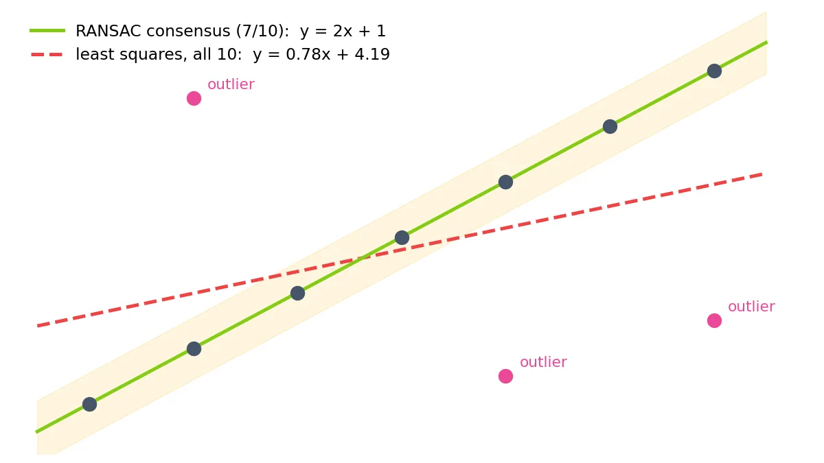
TL;DR — RANSAC (Random Sample Consensus) separates data into inliers and outliers while fitting a model: it fits a random minimal sample, counts how many points agree, and repeats until one sample wins by consensus. That simple loop is what makes findEssentialMat, solvePnPRansac and every panorama stitcher survive wrong matches. Three numbers tell the whole story: least squares over 10 detections with 3 false positives estimates a walking speed of 0.78 m/s when the truth is 2.00; RANSAC recovers the exact motion; and the required number of samples is governed by $N = \log(1-p)\,/\,\log(1 - w^s)$, which says 17 samples at 50% outliers for a 2-point line model but 1,177 for an 8-point model. On real data, an adjacent pair of temple photos from the SfM post has a 92% inlier ratio and needs about 5 samples; a near-opposite pair drops to 45% and needs 248.

RANSAC is an algorithm that separates a dataset into inliers, the measurements a single model explains, and outliers, the measurements it should ignore, and it estimates that model at the same time. The name, Random Sample Consensus, describes the whole method: draw a random sample of the data just big enough to determine a model, count its consensus (how many of the other points agree with it), and after enough draws keep the model with the most votes.

Computer vision leans on this constantly, because vision’s measurements come from detectors and matchers that are sometimes wrong rather than merely noisy: an object detector fires on a shadow, a feature matcher pairs two windows that happen to look alike. A single measurement like that can drag a least-squares fit arbitrarily far from the truth. The Structure-from-Motion article used RANSAC twice without opening it: once inside cv2.findEssentialMat, once inside cv2.solvePnPRansac. The camera-models post leaned on it for robust PnP. This post is the missing explanation. The algorithm is from 1981, fits in ten lines, and its design follows from one probability formula you can derive on a napkin [1].

The running example: reading a walking speed off the patio cam

The patio cam watches the garden path side-on, and this morning the courier crossed it at a steady walking pace. We want that pace from the camera alone. A person detector runs on one frame per second, the foot point of each bounding box is mapped to metres along the path (the ground-plane mapping the camera-models post calibrates), and out comes a list of $(t, x)$ measurements: at time $t$ seconds, a detection at $x$ metres. Constant speed means the true motion is a line,

$$x(t) = v\,t + x_0,$$

and in this clip the truth is $x = 2t + 1$: two metres per second, starting one metre in.

The detector is the weak link. It found the courier in all seven frames, but in three frames it also fired on something else: Bruno the garden gnome’s pointy hat at the 12-metre mark, a swaying shadow at 2 m, and a bush at 4 m. A missed detection would only leave a gap in the list, which costs nothing. A false positive injects a position that has nothing to do with the courier, and nothing in the data says which detection is which.

The full data, which every computation below uses:

courier detections	$(0,1)$ $(1,3)$ $(2,5)$ $(3,7)$ $(4,9)$ $(5,11)$ $(6,13)$
false positives	$(1,12)$ Bruno · $(4,2)$ shadow · $(6,4)$ bush

The catch: the algorithm receives all 10 detections with no labels. Nothing says which points are the courier and which are not.

Least squares averages the outliers in

The obvious move is a least-squares line fit over everything. Intuition for why it fails: least squares minimizes the sum of squared errors, so every point pulls on the answer, and a far-away point pulls hardest of all.

The idea: fit tiny, vote big

Fischler and Bolles turned the problem around in 1981 [1]. Instead of fitting one model to all the data, fit many models to the smallest possible subsets, and let the data vote:

1. Pick a minimal sample at random: the fewest points that determine the model. Two points for a line, three for a parabola. (Four matches for a homography, five for an essential matrix, eight for a fundamental matrix in the linear formulation.)
2. Fit the model to that sample alone.
3. Count the consensus: how many of all the points lie within a threshold $\tau$ of the model.
4. Repeat $N$ times and keep the sample with the largest consensus.
5. Refit the model by least squares on the winning consensus set. Outliers are no longer in the data, so least squares is now safe.

In pseudocode, the whole algorithm:

ransac(points, s, tau, N):
    best_model   = none
    best_inliers = {}
    repeat N times:
        sample  = s points drawn at random     # s = 2 for a line, 3 for a parabola
        model   = exact_fit(sample)            # uses the sample alone, no averaging
        inliers = { p in points : distance(p, model) < tau }
        if |inliers| > |best_inliers|:
            best_model, best_inliers = model, inliers
    best_model = least_squares_fit(best_inliers)   # final refit, now outlier-free
    return best_model, best_inliers

The distance function is whatever residual makes sense for the model: vertical distance to the line here, epipolar distance for an essential matrix, reprojection error for a pose. And the return value is half the point: alongside the model you get the split of the data into inliers (best_inliers) and outliers (everything else). In a pipeline that split is often the more valuable output; cv2.findEssentialMat returns exactly such a mask, and the SfM post used it to discard wrong matches before triangulating anything.

The trick is that a minimal sample either contains an outlier or it doesn’t. There is no averaging. A contaminated sample produces a wild line that few points agree with; a clean sample produces something close to the truth, and every inlier votes for it.

One wrinkle worth naming: the false positives only disagree because they have three different causes. Had the detector fired on Bruno in several frames instead, those detections would all sit at $x = 12$, and they would form their own consensus for the model $x(t) = 12$: a perfectly valid constant-velocity motion with $v = 0$. Self-consistent wrong measurements are the one thing voting cannot fix, and the Limitations section returns to them.

How many samples? The napkin derivation

RANSAC succeeds if at least one sample is all-inlier. That turns into an iteration count in three lines (both textbooks walk the same derivation: Szeliski §8.1.4 [2], H&Z §4.7 [3]). Let $w$ be the inlier fraction and $s$ the sample size. One sample is all-inlier with probability $w^s$; it fails with probability $1 - w^s$; $N$ independent samples all fail with probability $(1-w^s)^N$. Demand that this failure probability stay below $1-p$ for a target confidence $p$ and solve for $N$:

$$N \;=\; \frac{\log(1-p)}{\log(1 - w^s)}$$

The full table for $p = 0.99$, with the vision model each sample size corresponds to:

sample size $s$	model	$w=0.9$	$w=0.8$	$w=0.5$	$w=0.3$
2	line	3	5	17	49
3	parabola, P3P pose	4	7	35	169
4	homography	5	9	72	567
5	essential matrix	6	12	146	1,893
8	fundamental matrix (linear)	9	26	1,177	70,188

Read it by column and the message is that $w$ dominates: at 90% inliers everything is cheap, and at 30% inliers the big models are painful. Read it by row and you see why minimal solvers such as the five-point method matter enough to have their own papers: dropping $s$ from 8 to 5 at $w = 0.3$ cuts the work by 37×.

In practice $w$ is unknown, so implementations estimate it as they go: whenever a new best consensus appears, recompute $\hat{w}$ from it and shrink $N$ accordingly. The lab below runs this adaptive version.

The threshold is the other half

The consensus test needs a threshold $\tau$: how close must a point be to count as agreeing? This is the parameter that does not come from a formula. It encodes how much noise you expect on inliers. In the SfM pipeline, findEssentialMat used $\tau = 1.5$ px, meaning a match was accepted if it sat within 1.5 px of the epipolar geometry implied by the candidate model; PnP used a looser 4 px.

Both directions of error are real. Too tight, and noisy inliers fail the test, the consensus splinters, and the true model may never win. Too loose, and outliers start voting, until in the extreme every candidate gets full consensus and the winner is arbitrary. Push the threshold slider in the lab to both ends and watch each failure happen.

Now you try

Press Sample once a few times to see individual candidates and their bands, then Run RANSAC to let the adaptive loop finish and refit on the winning set. The amber dashed line is the candidate fitted to the two circled sample points, with its inlier band of width $\tau$; the blue line is the best consensus found so far; when the run completes, the green line is the least-squares refit on the winning inliers. Click the canvas to add outliers and watch $\hat{w}$ fall and $N$ climb. Then push the threshold to 0.1 and to 1.2 and see both failure modes from the paragraph above.

Same votes, curved model: calling a basketball shot

Nothing in the loop cares that the model is a line. Swap in a different model, its minimal sample size, and a distance function, and the algorithm carries over unchanged. The natural step up from the courier is a ball in flight, where the motion is a curve.

New scene: a phone films a basketball shot from the side, and a ball detector returns the ball’s centre in the frames where it finds one. Seen square-on, a ballistic arc is a parabola (air drag on a basketball over 4 m is small enough to ignore here; film it from an oblique angle and perspective bends it into a general conic, so we stay square-on, in metres). The model becomes

$$y(x) = a\,x^2 + b\,x + c,$$

three unknowns, so the minimal sample is now 3 points instead of 2. The question to answer before the ball arrives: does the fitted parabola pass through the hoop?

The detector found the ball in four frames and produced two false positives, one on a round ceiling light, one on a spare ball sitting on the rack. The rim of this backyard hoop is at $x = 4$ m and height 3.0 m, a touch under the regulation 3.05.

ball detections	$(0,2)$ $(1,3)$ $(2,3.5)$ $(3,3.5)$
false positives	$(1,5)$ ceiling light · $(2.5,1)$ rack ball

Two caveats belong to this example. Four detections is a toy; a real pipeline detects and tracks the ball across dozens of frames, and that fight is its own post, and the metrics for judging it are here. And a 99%-confidence RANSAC still fits a wrong model in 1 run out of 100, and the extrapolation to the rim magnifies whatever error the fit carries. The Limitations section returns to this.

The same votes on real photographs

The numbers above scale directly to the SfM pipeline’s data. Between two adjacent photos of the Middlebury temple ring, the ratio test passes 237 matches and RANSAC keeps 217 of them, an inlier ratio of $w = 0.92$. The essential matrix is a 5-point model, so the table says about 5 samples suffice for 99% confidence. That is why geometric verification of a thousand image pairs took seconds in the SfM post.

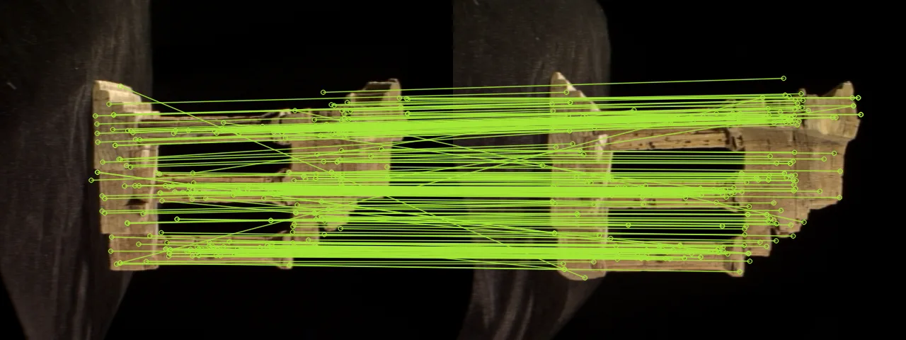
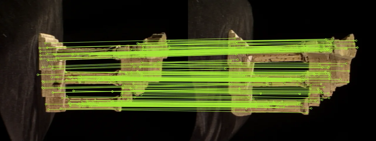
A pair from nearly opposite sides of the ring behaves differently: only 38 matches pass the ratio test and 17 survive RANSAC, $w = 0.45$, which needs about 248 samples. And with that few matches, honesty requires a caveat: a consensus of 17 among 38 could partly be luck, since with enough random trials some essential matrix will collect accidental agreement. Small consensus sets deserve suspicion, which is one of the limitations below.

Where RANSAC lives in the stack

Once you see the pattern, it is everywhere in this site’s pipelines. Essential matrix estimation in SfM §2: minimal sample of 5 matches, consensus by epipolar distance. Pose registration in SfM §5 and camera-models §5: solvePnPRansac, minimal sample of 3–4 correspondences, consensus by reprojection error. Homography estimation for panorama stitching, the subject of an upcoming post: minimal sample of 4. The model changes; the loop never does.

The modern descendants change the details while keeping the loop. MSAC/MLESAC score inliers continuously instead of counting them, so a barely-inside point counts less than a dead-center one [4]. LO-RANSAC adds a local refit whenever a new best appears, which recovers accuracy lost to minimal-sample noise [5]. MAGSAC++ removes the hard threshold entirely by marginalizing over it [6]. OpenCV ships all of this behind the USAC flags documented in [7]; cv2.USAC_MAGSAC is often a drop-in upgrade for the plain cv2.RANSAC flag.

Reproducibility

Parameter	Value
Toy numbers	the courier and basketball datasets are fully listed in their tables; least-squares fits via numpy.linalg.lstsq, the 3-point parabola solve via numpy.linalg.solve (numpy 2.2.4, Python 3.10.12)
Real match numbers	templeRing pairs (templeR0001+templeR0003 adjacent; templeR0001+templeR0024 near-opposite), SIFT + Lowe ratio 0.75, cv2.findEssentialMat(..., cv2.RANSAC, prob=0.999, threshold=1.5), OpenCV 5.0.0
Code	the sfm-from-scratch companion repo of the SfM post (match_pair / verify_pair in core/features.py)
Runs	OpenCV’s RANSAC is not seeded; the 217-inlier count was nevertheless identical across 3 consecutive runs on the adjacent pair. Counts on sparse pairs can vary run to run
N-table	every entry recomputable from $N = \lceil \log(1-p)/\log(1-w^s) \rceil$ with $p = 0.99$

Limitations & caveats

• The output is random. Two runs can return different models, and on hard data occasionally different answers. Seed the RNG when you need reproducibility, and treat single-run results accordingly.
• The formula is optimistic. $N$ assumes any all-inlier sample yields the true model. With noisy inliers, a minimal sample fits the noise of its 2–8 points, so the practical iteration count is higher than the table and the refit step is not optional. LO-RANSAC exists precisely because of this [5].
• Degenerate samples fit nothing. Two nearly-identical points define a meaningless line; five nearly-coplanar matches break the essential-matrix solver. Real implementations test samples for degeneracy before fitting.
• Consensus can be accidental. Repeated structure is the classic trap: on a building with identical windows, wrong matches between different windows are mutually consistent, and RANSAC happily verifies a wrong-but-popular model. A detector that keeps firing on the same stationary gnome builds a rival consensus at $v = 0$ the same way. Small consensus sets, like the 17/38 temple pair above, deserve suspicion.
• Extrapolation amplifies everything. The basketball call evaluates the fit a full metre past the last real detection, where the error in $a$ grows with $x^2$; the polluted fit missed the rim by 2.8 m. Even a clean consensus fit on noisy inliers drifts fastest outside the data, so predict as little beyond the observations as the application allows.
• The threshold is a modeling decision. It should reflect the inlier noise in the measurement (pixels of epipolar distance, reprojection error), and no formula in this post chooses it for you. MAGSAC++ is the current answer to removing it [6].
• It needs a parametric model. RANSAC verifies proposals; it cannot invent a model class. If the scene contains two people walking, it returns one of their motions, not both.
• Low inlier ratios get expensive fast. At $w = 0.3$ and $s = 8$ the table says 70,188 samples. Below roughly 20–30% inliers, plain RANSAC stops being the right tool and better matching, guided sampling, or a different formulation is needed.

Takeaways

• Least squares breaks under outliers because every point votes on every fit; on the patio data, 3 false detections in 10 turned a walking speed of 2.00 m/s into 0.78.
• RANSAC fits minimal samples and lets consensus decide, and it hands back the inlier/outlier split along with the model. A clean sample exists with probability $w^s$ per draw, and $N = \log(1-p)/\log(1-w^s)$ turns that into an iteration budget.
• Keep samples minimal: at 50% inliers, a line costs 17 samples and an 8-point model costs 1,177.
• The loop is model-agnostic: three points fit the basketball parabola instead of two for the line, and the same votes call the shot. Only the minimal solver and the distance function change.
• The threshold encodes expected inlier noise, and both too-tight and too-loose fail in ways you can reproduce in the lab.
• Always refit on the consensus set, and prefer cv2.USAC_MAGSAC over plain RANSAC in modern OpenCV [7].

Further reading

• The original paper: Fischler & Bolles [1] remains readable, and the application that motivated it was PnP under the name “location determination problem”.
• The textbook treatments: Szeliski §8.1.4 for the modern summary [2]; H&Z §4.7 for the estimation-theory view and the automatic-homography algorithm built around it [3].
• The state of the art: MAGSAC++ [6] and OpenCV’s USAC framework [7], which turn most of this post’s manual choices into library defaults.
• Related on CondadosAI: Structure from Motion from scratch (uses this twice) · camera models & PnP (robust PnP) · tracking metrics (how the basketball toy gets scored once it grows up) · next in this series: homogeneous coordinates, then bundle adjustment.

References

[1] Fischler, M. A., & Bolles, R. C. (1981). Random Sample Consensus: A Paradigm for Model Fitting with Applications to Image Analysis and Automated Cartography. Communications of the ACM, 24(6), 381–395. doi:10.1145/358669.358692

[2] Szeliski, R. (2022). Computer Vision: Algorithms and Applications (2nd ed.), §8.1.4 “Robust least squares and RANSAC” and §4.1.3 “Robust data fitting”. Springer. Free PDF

[3] Hartley, R., & Zisserman, A. (2004). Multiple View Geometry in Computer Vision (2nd ed.), ch. 4 “Estimation – 2D Projective Transformations”, §4.7 “Robust estimation”. Cambridge University Press. Book page

[4] Torr, P. H. S., & Zisserman, A. (2000). MLESAC: A New Robust Estimator with Application to Estimating Image Geometry. Computer Vision and Image Understanding, 78(1), 138–156. doi:10.1006/cviu.1999.0832

[5] Chum, O., Matas, J., & Kittler, J. (2003). Locally Optimized RANSAC. Pattern Recognition (DAGM 2003), Springer LNCS, pp. 236–243. doi:10.1007/978-3-540-45243-0_31

[6] Barath, D., Noskova, J., Ivashechkin, M., & Matas, J. (2020). MAGSAC++, a Fast, Reliable and Accurate Robust Estimator. CVPR 2020. doi:10.1109/cvpr42600.2020.00138 · arXiv:1912.05909

[7] OpenCV Documentation (4.12.0). USAC: Improvement of Random Sample Consensus in OpenCV. Docs