
fundamentals
31 posts · browse all tags
 Fundamentals
 An Image Is an Array: Shape, dtype, and Why OpenCV Hands You BGR
Lesson 1 of The Image as Data. One photograph, held three ways: a 24.7 MB mosaic of 12-bit counts, a 74.2 MB 16-bit development, and the 37.1 MB 8-bit array imread would give you. Two thirds of the numbers in that last one were never measured, adding 60 to a value of 207 gives 11, and a slice you write into changes the original.
 Fundamentals
 From Photons to Counts: What a Raw Number Means
A photosite collects electrons, a converter turns them into an integer, and that integer is all any algorithm ever sees. Measured on eighteen exposures of one scene: the count doubles with the shutter to within a few percent, then sticks near 3875 DN — and the ceiling the file declares is not the ceiling the sensor has.
 Fundamentals
 High Dynamic Range: Merging a Bracket, Then Checking It Against a Meter
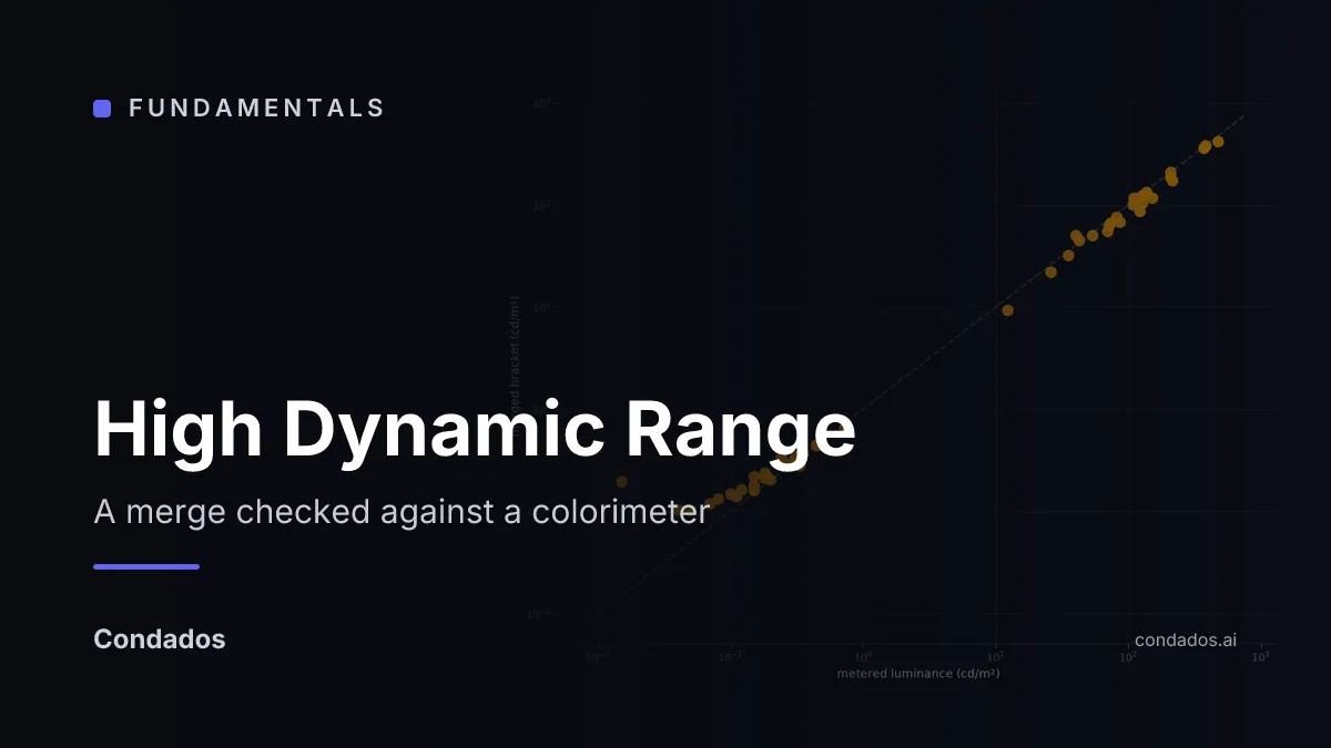
Eighteen exposures of a 17-stop scene, merged into one radiance map, calibrated with a single scale factor fitted on one patch — and then compared with the colorimeter readings taken in the room. The other 47 points land a median of 0.198 stops away, 0.109 stops across the neutral patches, and every large error is at the dark end.
 Fundamentals
 Image Formation: How a Camera Flattens the World Onto a Sensor
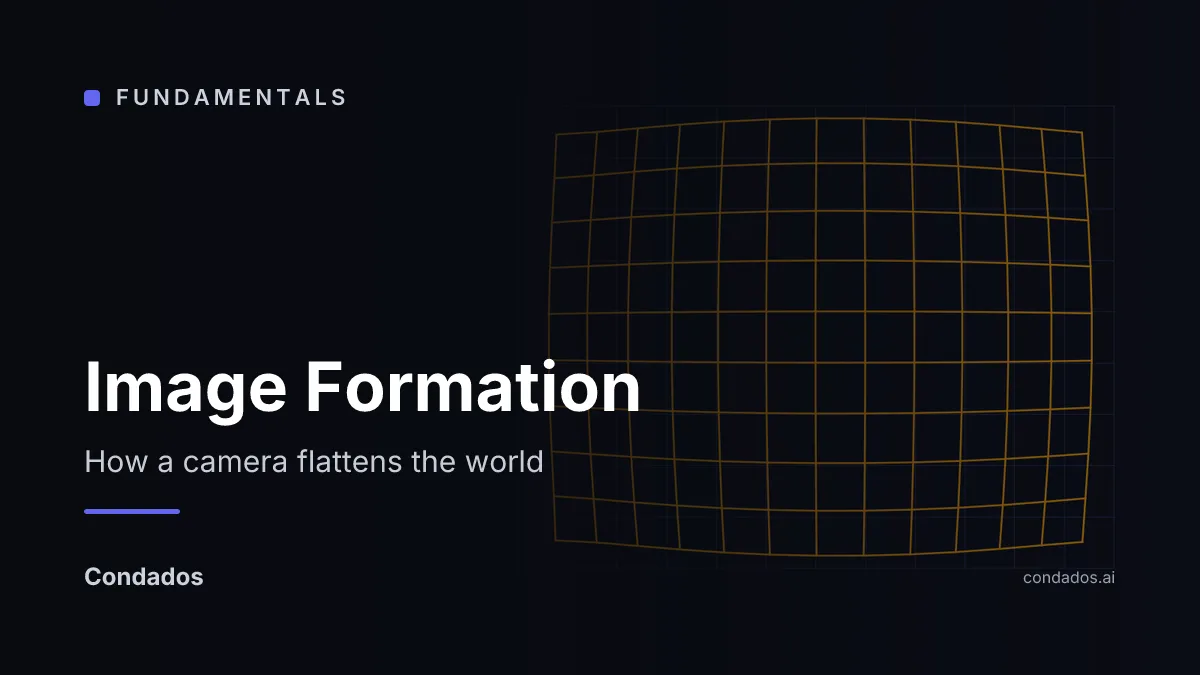
The unit overview: why a pinhole gives a sharp picture and a lens gives a bright one, what focus costs you, and where the pinhole model stops describing the lens in front of you. Measured on public photographs: a real lens moves a corner 51 px, stopping down from f/4 to f/22 deepens focus 5.54x, and a fisheye fitted with the wrong model misses by 7.3 px against 0.64 px with the right one.
 Fundamentals
 How Close Is Your Colour to the Real Thing?
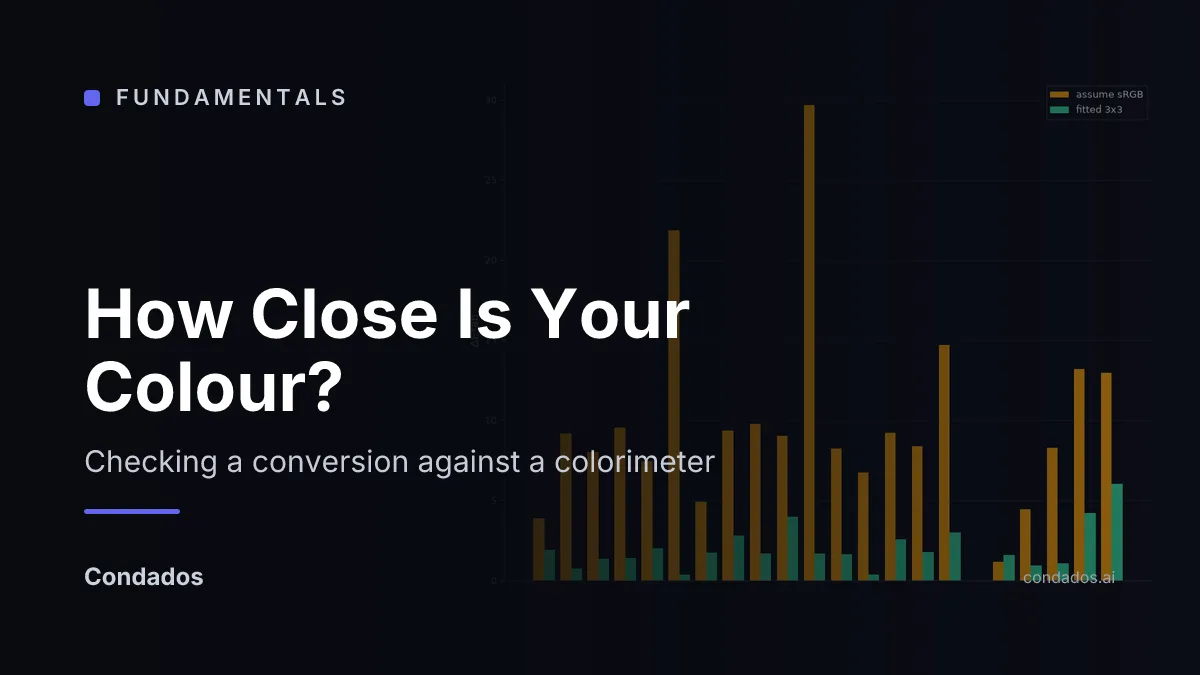
Lesson 5 of The Image as Data. Converting between colour spaces is exact arithmetic; deciding what the numbers mean physically is a fit. Checked against a colorimeter on 22 chart patches: treating the developed file as sRGB lands 9.54 ΔE*ab from the light in the room, the camera's own published matrix does no better, and a 3x3 fitted here and scored on patches it never saw reaches 2.41.
 Fundamentals
 File Formats: What the Encoder Did Before You Read the Pixels
Lesson 5 of The Image as Data. A JPEG quality sweep costs almost nothing in PSNR and takes Canny's edge agreement from 0.949 to 0.895. Chroma subsampling saves 40% of the bytes for 0.09 of ΔE. And OpenCV and Pillow decode every JPEG here bit-for-bit identically — the disagreement is a 16-bit PNG, which Pillow silently opens as 8-bit.
 Fundamentals
 Image Sensing: What the Number in a Pixel Actually Counts
The unit overview: how a photon becomes an integer, why that integer is a random variable, what the tone curve did to it before you saw it, and how eighteen exposures merge back into light you can put a unit on. Measured on one scene: gain 0.294 DN per electron, a full well near 13,200 e⁻, and a merged bracket that lands 0.109 stops from a colorimeter across the neutral patches.
 Fundamentals
 Lens Distortion: Where the Straight-Line Model Actually Fails
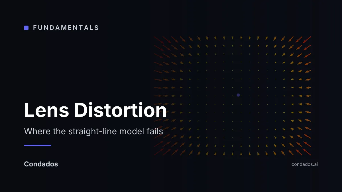
Lesson 3 of the Image Formation unit. Real glass bends rays more at the edges, and the error grows with the sixth power of radius. Measured on OpenCV's calibration set: the top-left pixel of a 640x480 frame belongs 51.22 px from where the pinhole model puts it, and adding the Brown-Conrady terms drops the mean reprojection error of one view from 2.55 px to 0.170 px. Straightening it back costs field of view rather than pixels: 61.67 degrees becomes 67.32.
 Fundamentals
 Lenses and Depth of Field: What You Buy With Light, and What It Costs
Lesson 2 of the Image Formation unit. A lens buys the brightness a pinhole cannot have and charges a plane of focus for it. Worked on a published scene: 93 mm at f/4 focused at 1.52 m is sharp from 1.500 m to 1.550 m, a band 5 cm deep. Stopping down to f/22 widens it to 0.277 m, a factor of 5.54 against an aperture ratio of 5.50, and the circle of confusion behind those numbers comes out at 0.0248 mm.
 Fundamentals
 The Pinhole Model: Why a Hole Makes a Picture, and Where the Prediction Fails
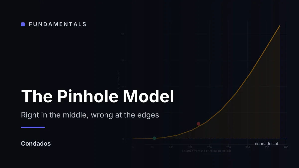
Lesson 1 of the Image Formation unit. A pinhole projects a scene point to a pixel by similar triangles, and that is a prediction you can check. Worked on one board corner from OpenCV's calibration set: the model puts it at (523.98, 77.94) and the detector found it at (513.77, 86.53), 13.34 px apart. Across the view the error is 0.29 px in the middle third of the frame and 5.75 px in the outer third, which is the shape of the problem the rest of the unit solves.
 Fundamentals
 Quantization: How Many Bits a Pixel Deserves
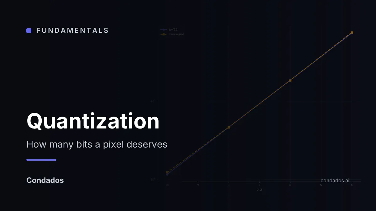
Lesson 3 of The Image as Data. Rounding to fewer levels costs Δ/√12 of error, and on this camera's mid-tones the formula predicts the measurement to within 2%. Set that error equal to the read noise unit 1.2 measured and the crossing lands at 9.3 to 9.5 bits — so a 12-bit file on this sensor carries about two and a half bits of nothing.
 Fundamentals
 Sampling: What One Pixel Covers, and What Falls Between
Lesson 2 of The Image as Data. One photosite on this camera is 5.527 µm and covers 1.056 arcminutes of the room. The table in the frame is ribbed at 7.4 pixels per cycle; keep every 8th pixel and it comes back at 96 pixels per cycle — thirteen times too coarse, and predicted exactly by folding the frequency.
 Fundamentals
 Sensing Colour: The Bayer Mosaic, and What Interpolation Costs
Lesson 5 of Image Sensing. A silicon photosite is colourblind, so a mosaic of filters gives each one a single colour — a quarter red, a quarter blue, half green. Two thirds of every colour image is therefore interpolated, and measured against photosites that actually exist, that guess costs 4.7 DN on a flat patch and 129.9 DN at an edge: twenty-eight times worse where it shows.
 Fundamentals
 Sensor Noise and Dynamic Range: Measuring the Gain You Were Never Told
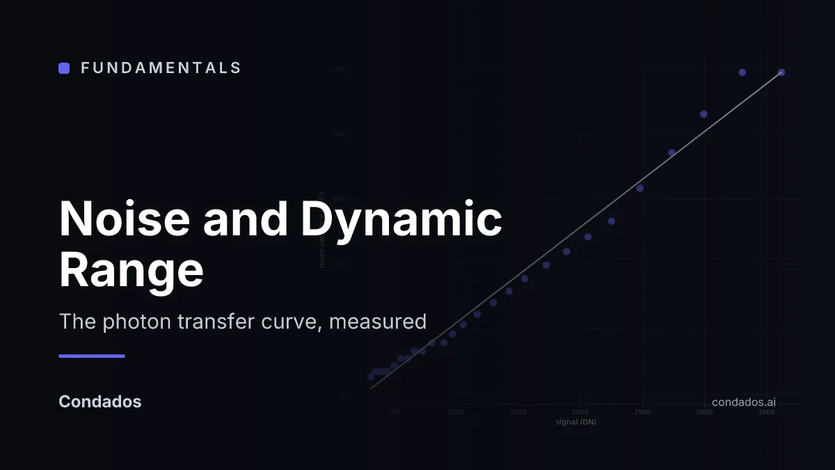
Read the same photosite three times and you get three numbers. Plotting the variance of a count against its mean gives a straight line whose slope is the sensor's gain: 0.294 DN per electron on this camera, R² = 0.986, a full well of 13,199 electrons and at least 11.21 stops of dynamic range — none of which appears anywhere in the file.
 Fundamentals
 The Camera Response Curve: Why Your JPEG Is Not Proportional to Light
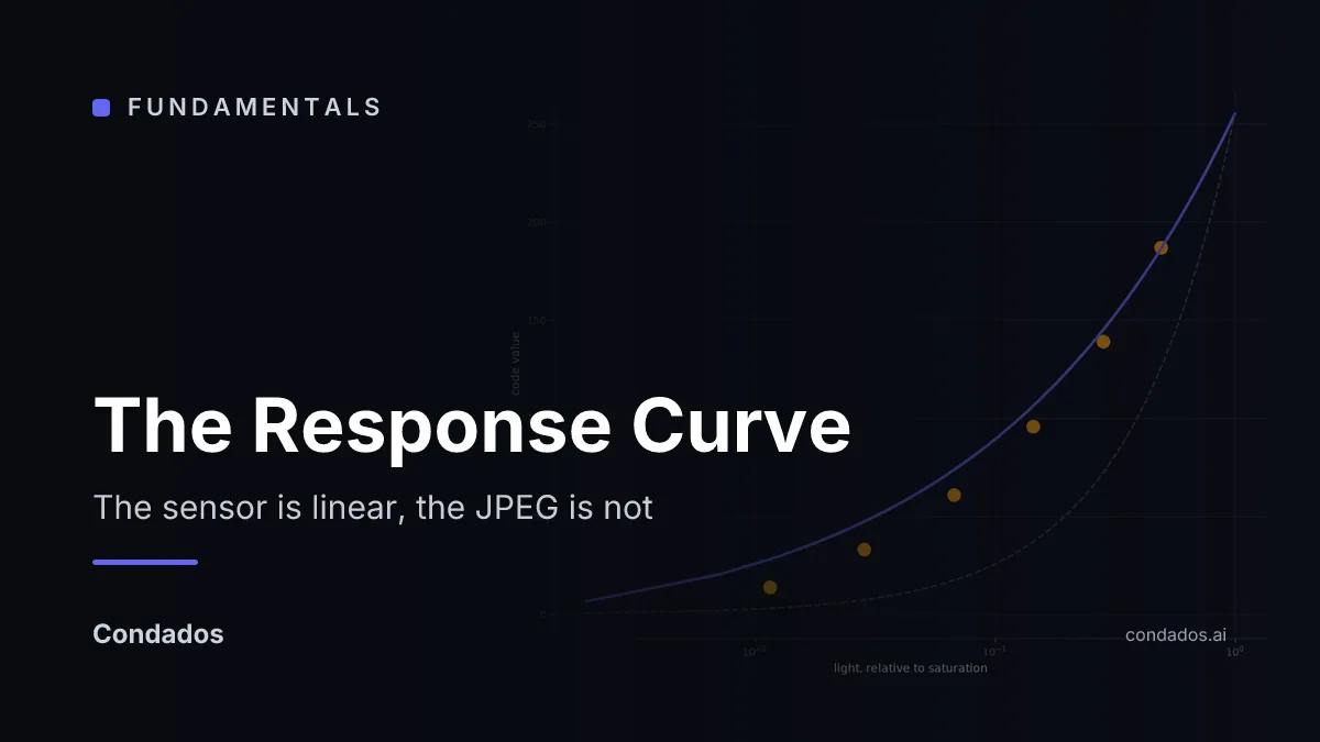
Raw counts are proportional to the light that arrived. The developed file is not: on the same six neutral patches, a linear ratio of 42 to 1 comes out as 187 against 14 code values. Measured here — a single exponent misses by 9.6 code values, because the curve is a gamma with a contrast S stacked on it.
 Fundamentals
 The Image as Data: The Grid, the Integers, the Axes, and the File
The unit overview: what an array actually holds, where its samples sit, how finely each one is written down, what its three numbers mean, and what the encoder did before you read any of it. Measured on one photograph: two thirds of a colour image is interpolated, a 7.4-pixel ribbing returns as 96-pixel banding when you decimate by eight, bit depth stops buying anything at 9.4 bits, and the naive route from file to colour lands 9.54 ΔE from the light in the room.
 Fundamentals
 Fisheye Models: When Correcting the Lens Stops Working
Lesson 4 of the Image Formation unit. Past roughly 120 degrees the pinhole model is not inaccurate, it is the wrong shape, because tan θ runs to infinity while the sensor does not. Fitted to the same 15 photographs of one fisheye lens, pinhole plus Brown-Conrady reaches 7.326 px RMS and Kannala-Brandt reaches 0.644 px. At 80 degrees the first model predicts a radius of -35,572 px, a sign flip; the second predicts 458.8 px, which is on the sensor.
 Fundamentals
 Canny: Non-Maximum Suppression and Hysteresis, Taken Apart
Lesson 4 of the Edge Detection unit. Canny is two independent mechanisms, not one tuned number. NMS collapses a five-pixel ridge to one pixel by comparing along the gradient; hysteresis keeps a weak chain because it touches a strong seed. Worked on nine numbers: a single threshold gives either 1 pixel or 9, and hysteresis gives the 6 that belong to a real contour. Measured on a photo, that is 204 contours averaging 18.68 px against 393 averaging 9.69 px at the same pixel budget.
 Fundamentals
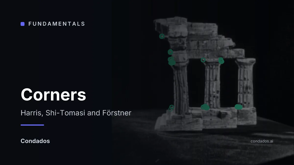
 Corners: The Structure Tensor, Harris, Shi-Tomasi and Förstner
Lesson 5 of the Edge Detection unit. A contour says where a boundary runs but not where you are along it. Two eigenvalues of a 2x2 matrix fix that: measured on a real photo, flat background scores 0.001/0.000, an edge 0.411/0.019 and a corner 0.442/0.318. Harris, Shi-Tomasi and Förstner all read that same matrix, and on the edge patch Harris comes out positive at k = 0.04 and negative at k = 0.06, so k decides the answer rather than the data.
 Fundamentals
 Edge Detection: Finding Where One Thing Stops and Another Begins
The unit overview: what counts as an edge, the two derivatives that find one, why a single threshold never works, and how contours become the points a matcher can use. Measured on one photo: smoothing across rows recovers 80% of the clean edge set at noise σ=20 against 63% without it, and hysteresis returns contours twice as long as a single threshold at the same pixel budget.
 Fundamentals
 Image Gradients: Central Differences, Prewitt and Sobel
Lesson 2 of the Edge Detection unit. Three operators compute the same derivative and behave differently on a noisy photo. Worked by hand on a 3x3 patch: Sobel gives Gx = Gy = 1.80, a magnitude of 2.55 and an orientation of 45 degrees, while Prewitt gives 1.20 and 1.70 on identical pixels. Measured across a noise sweep, Prewitt beats Sobel at every level, and the reason is that its normalised weights have a smaller sum of squares.
 Fundamentals
 The Laplacian, LoG and Zero-Crossings
Lesson 3 of the Edge Detection unit. The second derivative crosses zero at an edge instead of peaking, which locates a step edge at exactly x = 3.5 from integer pixels. It also has no smoothing in it: nine pixels disturbed by 0.03 produce four sign changes where there should be one. Measured on a photo, noise multiplies the zero-crossing pixels by 2.76x at sigma = 1.0 and 1.02x at sigma = 3.0, and only 33% of the resulting contours are closed.
 Fundamentals
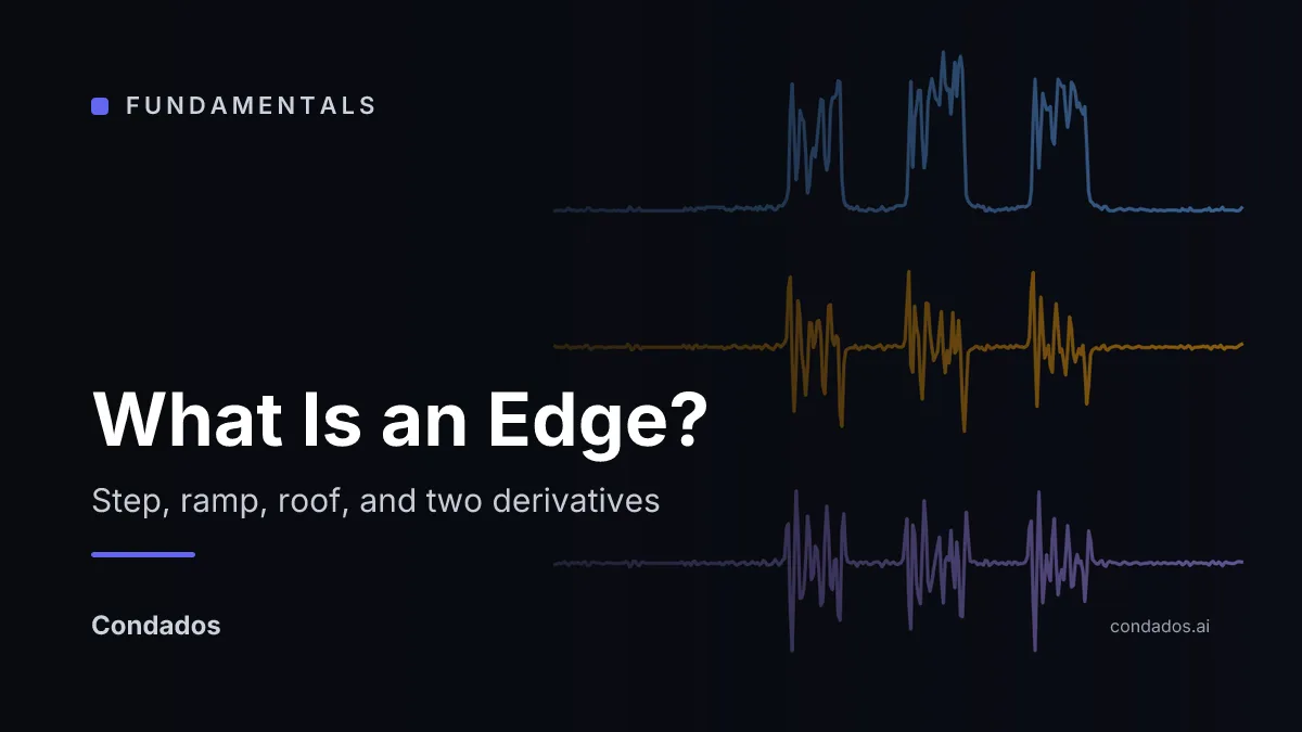
 What Is an Edge? Step, Ramp and Roof, and the Two Derivatives That Find Them
Lesson 1 of the Edge Detection unit. An edge is a peak in the first derivative and a sign change in the second. Worked by hand on nine pixels: the peak lands on column 4 and the second difference is exactly zero there. Add plus-or-minus 0.03 of noise and the first derivative holds its position while the zero-crossing slides half a pixel off the edge, which is why Canny is built on the first derivative and not the second.
 Fundamentals
 RANSAC: How Vision Algorithms Vote Away Outliers
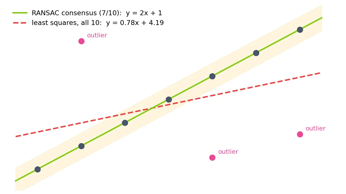
RANSAC separates data into inliers and outliers by fitting models to random minimal samples and keeping the one with the largest consensus. Walked end to end on two vision problems: a walking-speed estimate that three false detections drag from 2.00 m/s to 0.78, and a basketball shot called from a 3-point parabola fit. Plus the one-line formula for how many samples you need, a hands-on lab, and real inlier ratios measured on the temple dataset.
 Fundamentals
 What Makes a Point Matchable? SIFT, From Pixels to 128 Numbers
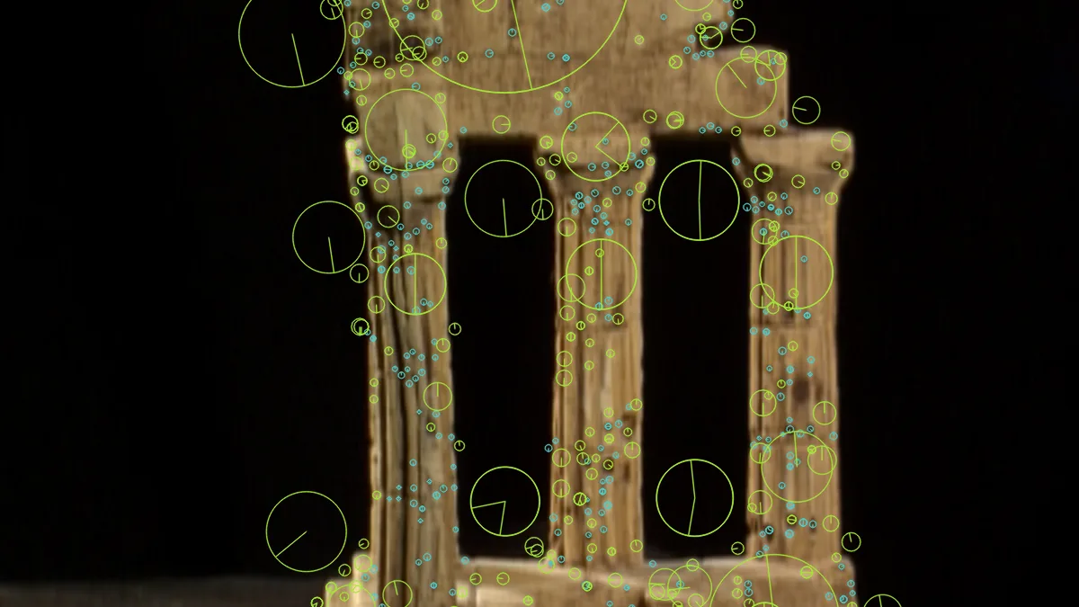
How SIFT turns a patch of pixels into 128 numbers that survive a moving camera. Measured on a real photo: a 45-level difference-of-Gaussians pyramid finds 791 keypoints spanning 1.8 to 112 px, each becomes a 128-dimensional descriptor, and Lowe's ratio test turns 791 candidates into 237 trustworthy matches. The invariances are real but bounded: 98.8% precision through a 45° rotation, and the scene is lost by 38° of viewpoint change. Every number has an artifact.
 Fundamentals
 Structure from Motion, from Scratch: 47 Photos to a 3-D Temple in ~800 Lines of Python
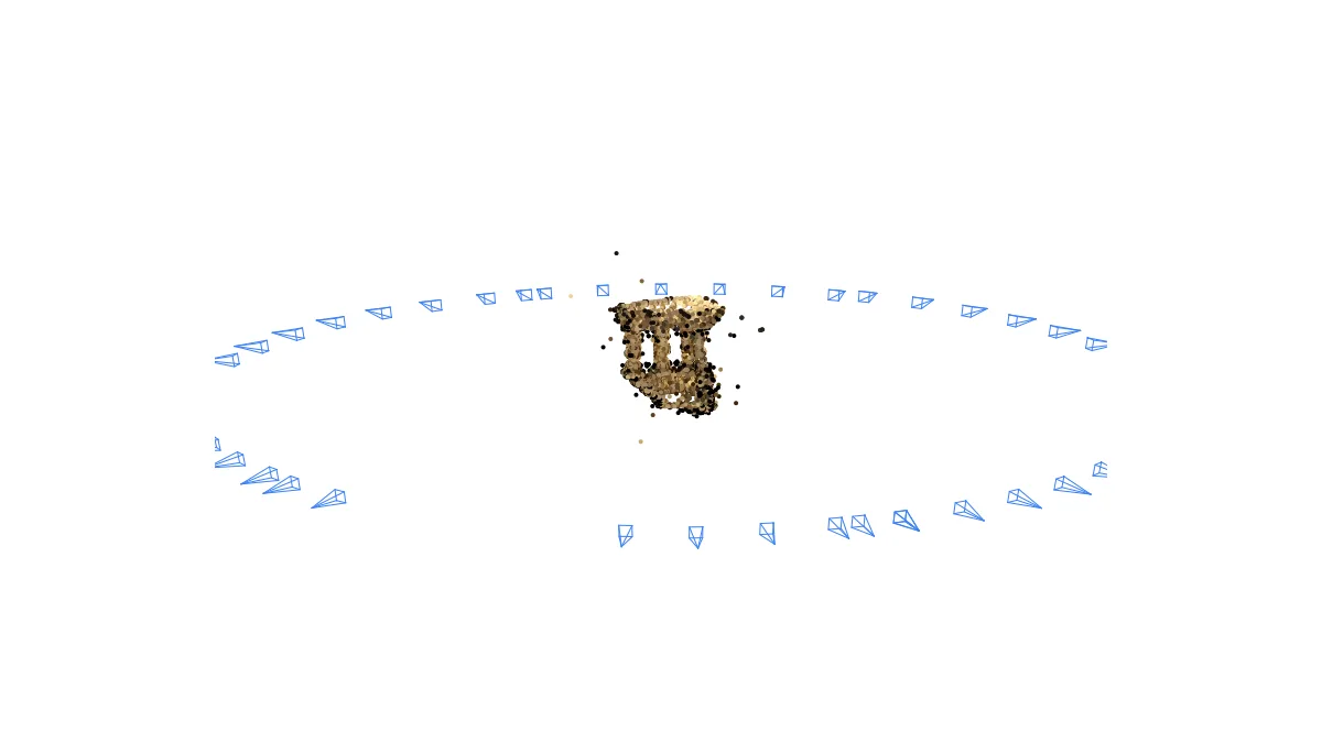
How overlapping 2-D photos become 3-D points and camera poses: SIFT matching, the essential matrix, triangulation, PnP growth, and sparse bundle adjustment, built from scratch with OpenCV + SciPy. The pipeline registers all 47 Middlebury temple views at 0.25 px mean reprojection error, next to COLMAP's 0.30 px on the same images. Worked examples, three interactive labs, and the reconstruction growing image by image.
 Fundamentals
 Camera Models, End to End: K, the Extrinsics, Calibration & PnP, with OpenCV
How a 3-D point becomes a pixel and back again: the intrinsic matrix K, the extrinsics R|t that place the camera in the world, Zhang calibration to 0.35 px reprojection error, and solvePnP recovering a 68-px-off pose to ~0. The math, two interactive labs, and runnable OpenCV in Python and C++.
 Fundamentals
 Image processing, computer vision, and computer graphics: one picture, three directions of the arrow
Three fields, one shared object: the digital image. Graphics turns a model into an image (forward), vision turns an image into a model (inverse), and image processing turns an image into a better image. Worked on a single red-ball scene, with a 1957→2026 timeline of how they split apart and re-merged.
 Fundamentals
 How 2D Convolution Works on Images: Kernels, Filters, and the Math, Interactively
2D convolution is the operation behind blur, sharpening, edge detection, and every CNN. Slide a kernel, multiply, sum: see it happen step by step in an interactive demo, apply real kernels to a live image, and get the math plus runnable OpenCV in Python and C++.
 Evaluation
 Classification Metrics, From the Ground Up: Precision, Recall, F1, ROC and AUC
The confusion matrix and everything that falls out of it: precision, recall, F1, specificity, the precision/recall trade-off, PR and ROC curves, and AUC, all built on one running toy example (a backyard cat-cam), with the equations, the intuition, and scikit-learn.
 Fundamentals
 Colour Spaces: Choosing Axes You Can Threshold
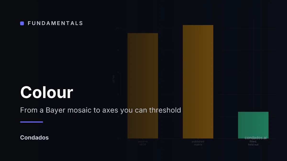
Lesson 4 of The Image as Data. A colour space is a choice of axes for the same three numbers, and the choice is what makes a question easy or impossible. Worked on one measured chart patch: RGB (149.8, 58.3, 34.0) becomes luma 82.8, hue 12 degrees stored as 6, and a Lab triple — plus the five-line red detector that is brittle in RGB and robust in HSV.