High Dynamic Range: Merging a Bracket, Then Checking It Against a Meter

No single exposure can hold a scene with a bright bulb and a deep shadow, but several exposures can, once each is divided by its own exposure time and they are averaged. Below, the eighteen exposures pass by, then settle on their merge.

You have used this merge:

• Phone HDR photos capture a quick burst at different exposures and merge them.
• Interior and real-estate photographers bracket a room so the window and the shadows both hold detail.
• HDR panoramas and light probes for 3-D rendering are built the same way.

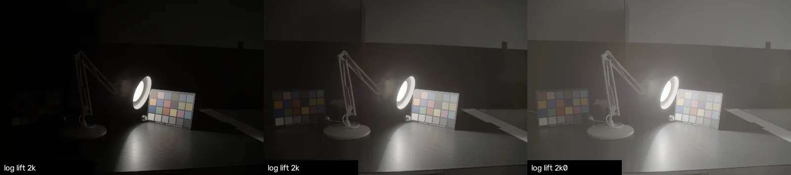
One exposure cannot hold this scene: at any shutter speed that shows the shadowed chart, the bulb has been clipped for ten stops. Eighteen exposures can, because each frame is proportional to light and divides out by its own exposure time. The result is one radiance map, and because someone stood in that room with a colorimeter, it is a result that can be marked: with a single scale factor fitted on one patch, the 48 chart patches (the anchor included) sit a median of 0.198 stops from the meter, and the twelve neutral patches a median of 0.109.

Where we are

Lesson 4 of image sensing. Lesson 1 said a raw count is proportional to light times exposure, lesson 2 measured what the count is made of, and lesson 3 showed why none of this works on the file a camera hands you. This lesson uses all three.

Why one frame is not enough

The scene spans 17.4 stops between the darkest metered patch, at 0.015 cd/m², and the brightest, at 2530 cd/m² [3]. Lesson 2 measured the sensor’s own range at about 11 stops. The gap is six stops, and no setting closes it.

The merge, in one line

Each frame gives a count $Z_i$ taken over a time $t_i$. Because raw is linear, the light that produced it is $Z_i / t_i$ up to a constant. Frames disagree only about which parts of the scene they can see: near the ceiling the count is clipped, near the floor it is mostly noise. Weight each frame by how much you believe it and average:

with $w$ a triangle that peaks in the middle of the usable range and falls to zero at both ends.

That is Debevec and Malik’s estimator [1] with the hard part removed. Their method recovers the response curve first, because they were working from photographs whose curve was unknown; with raw files there is no curve to recover, which is the practical payoff of lesson 3. OpenCV ships both halves, the merge and the calibration that goes in front of it when the input is not raw [5].

import numpy as np

weight_sum = np.zeros_like(planes[0], dtype=np.float64)
value_sum = np.zeros_like(weight_sum)
middle = (floor_dn + saturation) / 2

for plane, shutter in zip(planes, shutters):        # one colour channel per plane
    usable = (plane >= floor_dn) & (plane < saturation)
    weight = np.where(usable, 1.0 - np.abs(plane - middle) / (middle - floor_dn), 0.0)
    weight_sum += weight
    value_sum += weight * (plane / shutter)

radiance = np.divide(value_sum, weight_sum, out=np.zeros_like(value_sum), where=weight_sum > 0)

// OpenCV ships the same estimator, and its calibration step for the case where the
// response curve is unknown. On raw input the calibration is unnecessary.
std::vector<cv::Mat> images;         // the exposures
std::vector<float> times;            // their shutter speeds

cv::Mat radiance;
auto merge = cv::createMergeDebevec();
merge->process(images, radiance, times);   // add a CalibrateDebevec response for JPEGs

Giving it a unit

The merge produces relative radiance: correct ratios, arbitrary scale. A camera measures how much light arrived compared with the light next to it, and no photograph knows what a candela is. Turning ratios into cd/m² takes one number from an instrument.

Fairchild metered 54 points in the room with a Konica Minolta CS-100 at a 1° angle [3]. We fit one scale factor, on one patch: the lit chart’s white, at 382 cd/m². Every other point is then a prediction, and can be marked as one. This is the same shape as the survey’s own calibration, which normalises its published radiance maps with a single factor per scene.

Where the merge is wrong, and why

Every error above 1 stop is on the shadowed chart’s darkest patches, and all of them run in the same direction: the merge says there is more light than the meter did. Two causes fit that, and the obvious third suspect is ruled out by the data.

Flare. There is a bare bulb in the frame. Light scatters inside the lens and lands everywhere, including on the patches that should be nearly black. The meter, pointed at a patch from close range through a 1° aperture, does not see that scatter. It is a property of the optics, not of the sensor or the merge. I believe it is most of what the dark end of the table shows, but this scene gives no way to measure it separately.

Patch geometry, and one suspect meter point. The colorimeter measured a 1° spot; we average a rectangle inside the same patch. On a uniform patch that is the same quantity, and on a patch that is partly in the lamp’s shadow it is not. The worst point in the table may be a mismatch of this kind. On the lit chart, patch 3 meters ten times brighter than the black patch (127 against 12.3 cd/m²), and in the 30 s raw frame the shadowed chart’s patch 3 reads twice its black patch (1332 against 681 DN on the green channel). The meter says the opposite for the shadowed chart: 0.015 cd/m² for patch 3 against 0.04 for black. Flare can compress a ratio but it cannot invert one, so either the metered spot is not on that patch or the reading is off. The published data cannot say which, and the 3.72 stops on that patch should be read with that in mind.

Not the noise floor. It is the first suspect at the dark end, and the data rules it out. At 30 s the darkest shadowed patches (13 and 24) still read 681 DN on the green channel, with a measured noise variance of 110 DN², so a standard deviation of about 10.5 DN: 1.5% of the signal, and zero is some 65 standard deviations away. Nothing is clipped at zero or cut by the merge’s 24 DN floor at that level. It is the same point lesson 2 makes about why this scene cannot measure read noise: at 30 s nothing in it is dark.

Neither real cause is a reason to distrust the bright end, and both are reasons to report error by luminance decade rather than as one number.

Now you try

Take the eighteen exposures down to three and watch the shadow points fall off the bottom while the median error stays quiet. Then widen the spacing: the same number of frames covers more range and leaves holes in the middle.

What the phone in your pocket does instead

Bracketing assumes the scene holds still. Hand-held, it does not, and the standard answer since Hasinoff and colleagues at Google is to shoot a burst at one short exposure and merge the frames for noise instead of for range [2]. Averaging $N$ frames divides the noise by $\sqrt{N}$, which lifts the shadows out of the floor without ever risking a blown highlight, and alignment is a smaller problem than deghosting a bracket. The dynamic range comes from underexposing and then recovering the shadows, not from a long frame.

The arithmetic in this lesson is the same in both cases. What changes is which end of the range the extra frames are spent on.

In the wild

The bench scene needed eighteen exposures. Most photographs need one, and it is worth knowing which is which before reaching for a bracket.

Twilight over La Silla, in a single frame:

What it means: this scene did not need HDR. A photographer metered it, and the entire range from the lit dome to the darkest sky fits inside eight bits with 31 clipped pixels and sixty code values still spare. Bracketing it would have bought nothing.

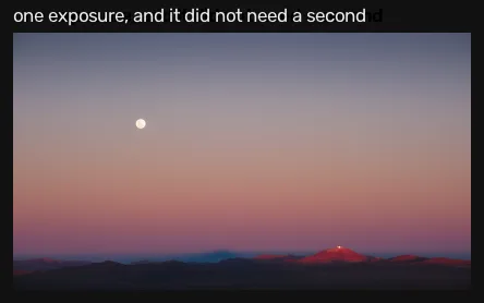
That is the counterweight to this lesson. The Luxo scene has a lit chart and a shadowed one nine stops apart, plus a bare bulb, and no single exposure holds it. A twilight landscape, for all its apparent drama, is a low-contrast subject: the sky is uniformly lit and the ground is uniformly dark. The question is never how dramatic a scene looks, it is how many stops separate the brightest thing you care about from the darkest, and the way to answer it is to take one frame and count what clipped.

Where this breaks

• A tone map is not a measurement. The pictures in this post are choices about how to show a radiance map on a screen; only the map has units. Reporting an HDR result as a tone-mapped image hides everything this lesson measured, and the literature on doing it well is a book in itself [4].
• One scale factor is doing real work. The check is of the shape of the reconstruction, not its absolute level: the level was given by the meter. Without an instrument, a merged bracket is still only relative light.
• The scene is static and on a tripod. No ghosting, no alignment, no moving subject. Real bracketing spends most of its difficulty there, and none of it appears here.
• The comparison is against the survey’s own colour matrix, fitted by Fairchild on this scene’s lit chart [3]. Errors in that matrix show up as errors in our luminance, especially on saturated patches, which is why the neutral-patch figure (0.109 stops) is quoted separately from the all-patch one (0.198).
• Green alone gives 0.264 stops. Using a single channel instead of a luminance-weighted combination raises the median error from 0.198 to 0.264 stops, 0.066 stops worse. The artifact records only that median, so how the cost splits between neutral and saturated patches is not measured here.

Next

The merge in this lesson ran on four channel planes, R, G1, G2 and B, and combined them with a borrowed matrix row as if each colour were there at every pixel. It is not: each photosite measured one of them. Lesson 5 is where the channels come from, and what it costs to fill in the two thirds of a colour image that no photosite measured.

References

[1] Debevec, P. E., & Malik, J. (1997). Recovering high dynamic range radiance maps from photographs. SIGGRAPH ‘97, pp. 369–378. doi:10.1145/258734.258884

[2] Hasinoff, S. W., Sharlet, D., Geiss, R., Adams, A., Barron, J. T., Kainz, F., Chen, J., & Levoy, M. (2016). Burst photography for high dynamic range and low-light imaging on mobile cameras. ACM Transactions on Graphics, 35(6), 1–12. doi:10.1145/2980179.2980254

[3] Fairchild, M. D. (2007). The HDR Photographic Survey. Proceedings of the IS&T 15th Color and Imaging Conference, pp. 233–238. doi:10.2352/CIC.2007.15.1.art00044. The scene, its 54 metered points, and the D2x characterisation whose luminance row is used here: markfairchild.org/HDRPS/HDRcharacterization.html. Used for research and non-commercial publication, as its terms require.

[4] Reinhard, E., Heidrich, W., Debevec, P., Pattanaik, S., Ward, G., & Myszkowski, K. (2010). High Dynamic Range Imaging: Acquisition, Display, and Image-Based Lighting (2nd ed.). Morgan Kaufmann. The book-length treatment of capture, encoding and tone reproduction.

[5] OpenCV Documentation (5.0). Computational photography: HDR imaging: createMergeDebevec, createCalibrateDebevec and the tone-mapping operators. docs.opencv.org/5.0