
Fisheye Models: When Correcting the Lens Stops Working
Lesson 4 of the Image Formation unit. Past roughly 120 degrees the pinhole model is not inaccurate, it is the wrong shape, because tan θ runs to infinity while the sensor does not. Fitted to the same 15 photographs of one fisheye lens, pinhole plus Brown-Conrady reaches 7.326 px RMS and Kannala-Brandt reaches 0.644 px. At 80 degrees the first model predicts a radius of -35,572 px, a sign flip; the second predicts 458.8 px, which is on the sensor.
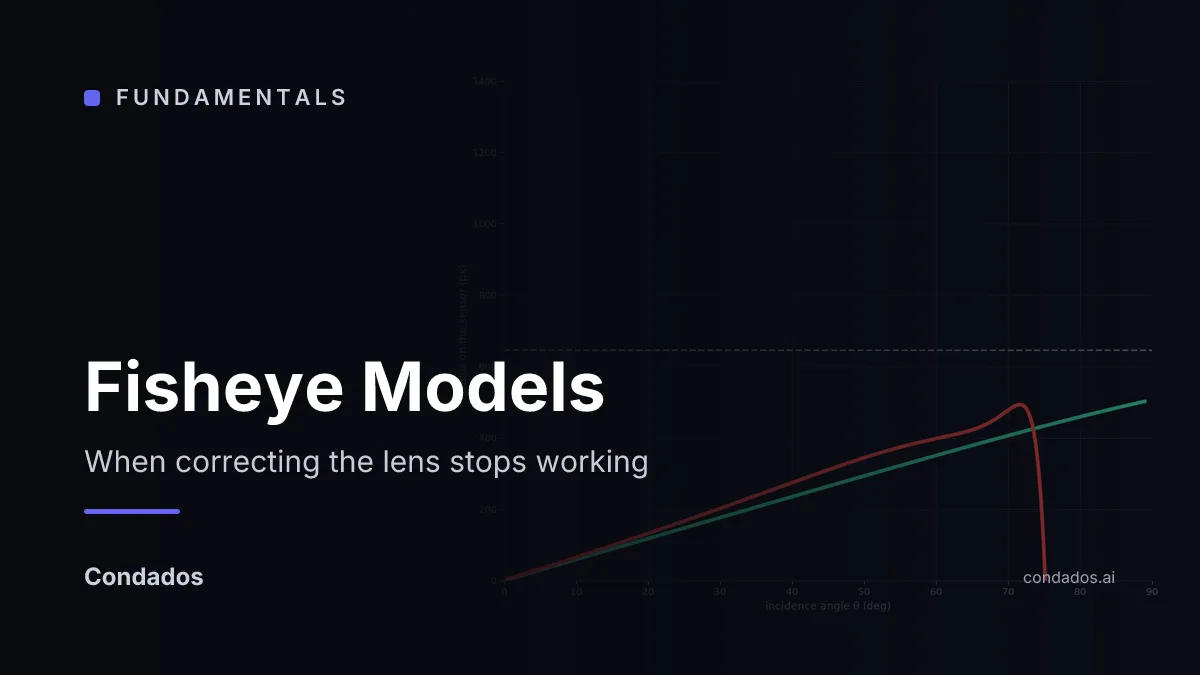
Everything in this unit so far corrects a model in which a ray at angle lands at . That quantity runs to infinity as approaches 90°, and a sensor does not, so no polynomial correction can describe a lens that sees past about 120°. Fitted to the same 15 photographs of one fisheye lens, the pinhole model plus Brown–Conrady reaches 7.326 px RMS where Kannala–Brandt reaches 0.644 px.
Where we are
Lesson 4 of image formation, and the last. Lesson 3 corrected a real lens to 0.170 px with five coefficients, and ended on the ceiling built into that correction: the thing being corrected is .
The unit’s second lens is where that ceiling is visible. It is a fisheye, and the measurements below come from 15 photographs of a board with 6×8 interior corners at 1032×778.
The tangent is the problem
Intuition first: the pinhole model puts a flat image plane in front of the camera, and asks where a ray pierces it. A ray arriving at 89° is very nearly parallel to that plane, so it pierces it a very long way out. At exactly 90° it never does. That is not a defect of a particular lens; it is what a flat image plane means, and it puts a hard limit under 180° on any camera that uses one [2].
A fisheye lens is built to a different rule. Rather than preserving straight lines, it maps angle to radius directly, and the common designs differ only in how:
Every one of them is finite at 90° and beyond. Rather than pick one, Kannala and Brandt [1] fit an odd polynomial in , which contains all of them as special cases:
This is what cv2.fisheye implements, with four coefficients rather than the five
of Brown–Conrady [3]. The change is not that there are different numbers
of terms. It is that the polynomial multiplies instead of .
One ray, two models
Across the range the two predictions stay within 11% of each other out to 15° and 17% out to 45°, both still climbing, and then one of them stops being a position at all:
| θ | pinhole + Brown–Conrady | Kannala–Brandt |
|---|---|---|
| 15° | 98.4 px | 88.2 px |
| 45° | 309.9 px | 263.9 px |
| 60° | 397.6 px | 350.3 px |
| 70° | 477.2 px | 406.1 px |
| 80° | −35,572 px | 458.8 px |
| 89° | −8.3 × 10¹¹ px | 502.1 px |
The consequence for the fit is the number this lesson exists for. On the same 15 views, with the same corners:
| Model | RMS reprojection error | Worst view |
|---|---|---|
| Pinhole + Brown–Conrady | 7.326 px | 10.434 px |
| Kannala–Brandt | 0.644 px | 1.247 px |
A factor of 11.4. Both models were given identical data and identical corner locations; the only difference is what they assume happens between the world and the sensor.
Now you try
Start at 60°, where the models still look like variations on a theme, then drag toward 89 and watch the perspective readout leave the sensor and then the plot entirely. The fitted Kannala–Brandt curve sits almost on top of the equidistant line, which is what a well-behaved fisheye looks like.
One difference from the table above, so the numbers do not look contradictory: the lab draws all five models at one shared focal length, because the question it answers is what the five shapes do. The table gives each model the focal length it was actually fitted with, 372.22 px for the pinhole and 336.86 px for the fisheye, so its perspective row is smaller than the lab’s at the same angle.
Fitting one, in practice
import cv2, numpy as np

h, w = gray.shape
# Without a starting guess the solver converges to a focal length it cannot
# recover from. f = max(w, h) / pi is the equidistant estimate for a 180 degree lens.
k = np.array([[max(w, h) / np.pi, 0, w / 2], [0, max(w, h) / np.pi, h / 2], [0, 0, 1]])
flags = cv2.CALIB_USE_INTRINSIC_GUESS | cv2.CALIB_RECOMPUTE_EXTRINSIC | cv2.CALIB_FIX_SKEW
rms, k, d, rvecs, tvecs = cv2.fisheye.calibrate(
    obj_points, img_points, (w, h), k, np.zeros((4, 1)), None, None, flags
)
#include <opencv2/opencv.hpp>
// Without a starting guess the solver converges to a focal length it cannot
// recover from. f = max(w, h) / pi is the equidistant estimate for a 180 deg lens.
const double f0 = std::max(size.width, size.height) / CV_PI;
cv::Mat K = (cv::Mat_<double>(3, 3) << f0, 0, size.width / 2.0,
0, f0, size.height / 2.0,
0, 0, 1);
cv::Mat D = cv::Mat::zeros(4, 1, CV_64F);
const int flags = cv::CALIB_USE_INTRINSIC_GUESS |
cv::CALIB_RECOMPUTE_EXTRINSIC | cv::CALIB_FIX_SKEW;
const double rms = cv::fisheye::calibrate(objPoints, imgPoints, size, K, D,
cv::noArray(), cv::noArray(), flags);Two details in that snippet cost an afternoon each. The intrinsic guess is not
optional: left to initialise itself, the solver settles 200 px from the corners
on this lens, and seeding it with is the difference between a
fit and a failure. And in OpenCV 5 the flags moved out of the cv2.fisheye
namespace into cv2, so every tutorial written against 4.x raises AttributeError
on that line.
In the wild
A circular fisheye makes a testable promise: under the equidistant model, radius on the sensor grows linearly with angle, . At the edge of a 180° field , so the image circle’s radius should be — a number that follows from the focal length alone.
A Canon EOS 6D with the EF 8–15 mm at 8 mm, the frame cropped square, so its height is the sensor’s 24 mm short side and the pixel pitch is fixed at 6.579 µm:
Thresholding the exposed disc against the black corners gives a measured radius of 1752 px — 91.7% of the prediction.
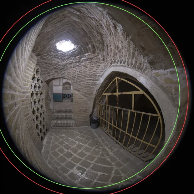
What it means: eight per cent is a good result and an honest one. The gap has more than one candidate and this measurement cannot separate them: the EF 8–15 mm is not exactly equidistant, the square crop may not be centred on the optical axis, and the disc’s edge is a soft vignette rather than a line. Naming one of those as the cause would need a calibration target, which is the next lesson’s business rather than this one’s. The useful figure to carry away is the scale: 4.71° of the world per 100 pixels, everywhere in the frame, which is exactly what an equidistant projection buys you.
Where this breaks
Rectifying a fisheye to a pinhole gives back the problem you started with. The obvious next step is to undistort into a rectilinear image, and it is available. But the output is a flat image plane again, so the field of view past about 120° has nowhere to go: either it is cropped away, or the corners are stretched across so many pixels that nothing is left of the detail. Real fisheye pipelines keep the fisheye model and work in it.
CALIB_CHECK_COND rejects most of a usable dataset. Turned on, OpenCV’s
conditioning check throws out 12 of these 15 views, while the fit over all 15
converges to 0.644 px. The check is not measuring what it sounds like it measures,
and a pipeline that silently drops views on its advice is calibrating on a third of
its data.
The polynomial is not guaranteed to be monotonic. Nothing in the fit forces to keep increasing with , and a badly conditioned set of coefficients can fold the outer field back on itself, exactly as the pinhole model does here at 80°. Sanity-check the fitted curve over the whole range rather than trusting a low RMS, which is an average over the corners you happened to observe.
And the coefficients describe this lens only. These four numbers came from one lens photographed 15 times. They are not “the fisheye correction”, and using them on another camera is worse than using no correction at all.
The unit ends here
Four lessons, one thread: a hole makes a picture, a lens makes it bright, real glass bends the geometry, and past a certain field of view the geometry is a different one. The unit’s hub has the summary and the shared references, and the next thing worth reading is camera models, calibration and PnP, which takes these two scalar equations and turns them into the matrix that geometry is written in.
Run it: every code block on this page has a cell in the unit’s notebook — open it in Colab.
References
[1] Kannala, J., & Brandt, S. S. (2006). A Generic Camera Model and Calibration Method for Conventional, Wide-Angle, and Fish-Eye Lenses. IEEE Transactions on Pattern Analysis and Machine Intelligence, 28(8), 1335–1340. doi:10.1109/TPAMI.2006.153
[2] Hartley, R., & Zisserman, A. (2004). Multiple View Geometry in Computer Vision (2nd ed.), ch. 6 “Camera Models”, §6.4 “Other camera models” (p. 174). Cambridge University Press.
[3] OpenCV Documentation (5.0). Fisheye camera model (cv::fisheye). docs.opencv.org/5.0