Lens Distortion: Where the Straight-Line Model Actually Fails

Lesson 3 of the Image Formation unit. Real glass bends rays more at the edges, and the error grows with the sixth power of radius. Measured on OpenCV's calibration set: the top-left pixel of a 640x480 frame belongs 51.22 px from where the pinhole model puts it, and adding the Brown-Conrady terms drops the mean reprojection error of one view from 2.55 px to 0.170 px. Straightening it back costs field of view rather than pixels: 61.67 degrees becomes 67.32.

Luis Condados · August 19, 2026

computer-vision camera-calibration opencv optics fundamentals

The displacement the lens applies to every point in the frame. Near zero at the principal point, unmissable at the corners.

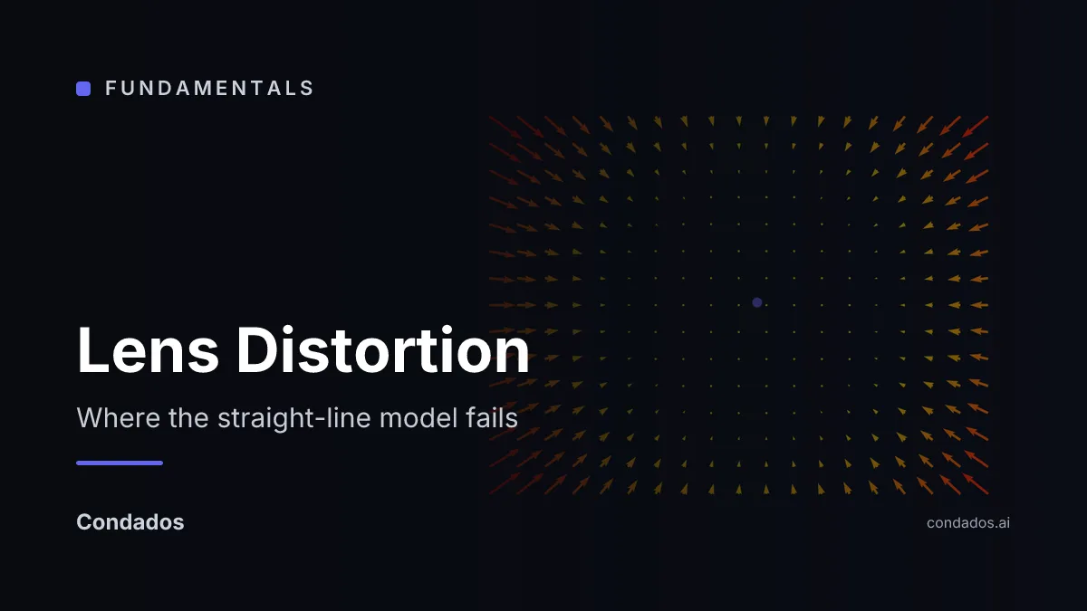
A real lens bends rays more the further from its axis they arrive, so the pinhole model is right in the middle of the frame and wrong at the edges. On the unit’s camera the top-left pixel sits 51.22 px from where the straight-line model puts it, while a pixel 38 px from the centre is off by 0.04 px. Adding five coefficients drops one view’s mean error from 2.55 px to 0.170 px. Undistorting the result does not crop the image; it costs field of view, 61.67° becoming 67.32°.

Where we are

Lesson 3 of image formation. Lesson 1 left a residual it could not explain: projecting board corners with the two scalar equations was accurate to 0.29 px near the middle of the frame and off by 5.75 px near its edges. Lesson 2 explained what the lens buys, assuming it bends every ray by exactly the right amount. It does not, and the difference is what lesson 1 measured.

The error is radial, so the model is a function of radius

Intuition first: a simple lens is a piece of glass with spherical surfaces, and the angle a ray is bent through depends on where it strikes that surface. Rays arriving near the rim meet a steeper curve than rays near the middle, so they are bent too much. Nothing about that depends on the direction the ray came from, only on how far off-axis it lands, which is why the correction is written as a function of radius alone [2].

Work in coordinates centred on the optical axis and scaled by focal length, so the image is described independently of its resolution:

x = \frac{u - c_x}{f_x}, \qquad y = \frac{v - c_y}{f_y}, \qquad r^2 = x^2 + y^2.

The Brown–Conrady model [1] then multiplies by an even polynomial in $r$ and adds two small terms for a lens that is not perfectly parallel to the sensor:

x_d = x\,(1 + k_1 r^2 + k_2 r^4 + k_3 r^6) + 2p_1 x y + p_2 (r^2 + 2x^2),

y_d = y\,(1 + k_1 r^2 + k_2 r^4 + k_3 r^6) + p_1 (r^2 + 2y^2) + 2p_2 x y.

Only even powers appear, because a lens has no reason to treat one side differently from the other. The polynomial equals 1 at $r = 0$ , so the centre of the image never moves no matter how bad the lens is.

Worked example · The top-left pixel of left01.jpg

Calibrating the unit’s 13 photographs gives $k_1 = -0.2651$ , $k_2 = -0.0467$ , $k_3 = 0.2523$ , $p_1 = 0.00183$ , $p_2 = -0.00031$ . Take the pixel at $(0, 0)$ , the extreme corner, and normalise it:

x = \frac{0 - 342.37}{536.07} = -0.63866, \qquad y = \frac{0 - 235.54}{536.02} = -0.43942

r^2 = 0.60098, \qquad r = 0.77523

The three radial terms, individually:

k_1 r^2 = -0.15931, \qquad k_2 r^4 = -0.01688, \qquad k_3 r^6 = +0.05477

so the radial factor is $1 - 0.15931 - 0.01688 + 0.05477 = 0.87857$ . The two tangential terms contribute 0.000583 to $x_d$ and 0.001633 to $y_d$ , which is roughly a thousandth of what the radial part does. Multiplying back into pixels:

u_d = 342.37 + 536.07 \times (-0.56053) = 41.89, \qquad v_d = 235.54 + 536.02 \times (-0.38443) = 29.48

What it means: the scene content that the straight-line model says belongs at the very corner $(0,0)$ actually lands at $(41.89, 29.48)$ , which is 51.22 px away. The radial factor being less than 1 is barrel distortion: everything is pulled toward the centre, so the corners of the world are squeezed inward. And the tangential terms earn about a tenth of a pixel on this lens, which is a fair description of how much sensor tilt it has.

The whole behaviour is in that $r^6$ : the displacement is negligible for most of the frame and then climbs steeply.

Distance from the principal point	Displacement
38 px	0.04 px
115 px	1.35 px
192 px	6.37 px
269 px	17.23 px
345 px	33.94 px
384 px	43.06 px

The same lens, measured along the diagonal. Out to about a quarter of the way the straight-line model is right to a pixel; past halfway the two curves have nothing to do with each other.

Now you try

The lab opens on this camera’s measured coefficients. Drag $k_1$ toward zero and the red grid straightens; push it positive and the bow reverses into pincushion. The tangential sliders are worth a moment too: they have to be pushed a hundred times past this lens’s values before they do anything visible.

Try it: bend the lens

Undistorting costs field of view, not pixels

With the coefficients known, the correction is one OpenCV call, and for video the map is worth precomputing once [3]:

import cv2

undistorted = cv2.undistort(img, K, dist)          # one frame

h, w = img.shape[:2]                                # for video, build the map once
new_k, _ = cv2.getOptimalNewCameraMatrix(K, dist, (w, h), 0)
map1, map2 = cv2.initUndistortRectifyMap(K, dist, None, new_k, (w, h), cv2.CV_16SC2)
undistorted = cv2.remap(img, map1, map2, cv2.INTER_LINEAR)

#include <opencv2/opencv.hpp>

cv::Mat undistorted;
cv::undistort(img, undistorted, K, dist);           // one frame

cv::Mat map1, map2;                                  // for video, build the map once
cv::Mat new_k = cv::getOptimalNewCameraMatrix(K, dist, img.size(), 0);
cv::initUndistortRectifyMap(K, dist, cv::noArray(), new_k, img.size(),
                            CV_16SC2, map1, map2);
cv::remap(img, undistorted, map1, map2, cv::INTER_LINEAR);

The usual warning is that undistortion crops the image. On this lens it does not. Counting output pixels with no source pixel to read from:

New camera matrix	Horizontal field of view	Output with no source
the same $f$	61.67°	0.00%
`alpha = 0`	67.32°	0.03%
`alpha = 1`	68.56°	5.15%

Keeping the same focal length wastes nothing and shows 61.67°, while the lens actually collected 67.32°. Barrel distortion squeezes the outer scene inward, so the pixels are there; correcting at the same $f$ pushes them off the edge. Asking OpenCV for the widest view that is still fully covered recovers those 5.65° for 0.03% empty output. The trade is field of view against black corners, not sharpness against area.

In the wild

Vignetting is easy to assert and awkward to measure, because you need a subject that is genuinely uniform. A brick wall photographed square-on is close enough: it fills the frame, it is flat, and it was lit by the sky.

Sampling a patch at the centre and one in each corner of a compact camera’s frame:

	code value
centre	133.4
top left	123
top right	115
bottom left	129
bottom right	115

The worst corner sits at 85.9% of the centre, which is 0.22 stops of falloff.

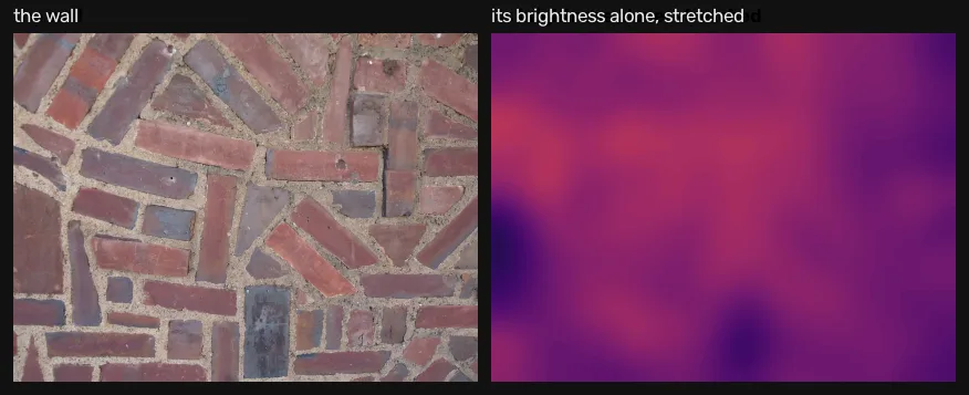
A brick wall, and beside it the same wall reduced to its slowly-varying brightness, stretched so that the corner falloff is visible — The wall, and its brightness alone with the texture blurred away and the scale stretched. A fifth of a stop is invisible in the photograph and unmistakable once the bricks are removed. Source: “Surfaces brick wall with unstandard pattern” by Tomwsulcer (Wikimedia Commons), CC0.

What it means: 0.22 stops is small — this is a modest zoom at a middling aperture, not a fast prime wide open, where two stops in the corners is ordinary. But small is not zero, and the sign of the error is always the same. Stack a hundred frames for a panorama and the seams show; measure reflectance across a field and the edges read dark; flat-field a microscope image without correcting it and every measurement inherits the same bias.

Where this breaks

The polynomial is a fit, not a law. $k_3$ especially is often noise: with a board that does not reach the corners of the frame there is nothing constraining the $r^6$ term, and fitting it anyway can make predictions worse outside the region that was measured. OpenCV provides CALIB_FIX_K3 for exactly this reason, and a calibration whose coefficients change a lot when you add images has not converged.

Everything above assumes the distortion is radial about one centre. Vignetting, the darkening toward the corners, is also radial but acts on brightness rather than position, so none of these coefficients touch it. Chromatic aberration is worse for this model: red and blue focus at different distances, so the correct displacement differs per channel, and a single set of coefficients fitted on greyscale corners splits the difference.

And the model has a hard ceiling. Everything here is a correction to $x = X/Z$ , which is $\tan\theta$ for a ray arriving at angle $\theta$ . As $\theta$ approaches 90° that tangent runs to infinity, so no polynomial in $r$ can describe a lens that sees past about 120°. Fitting this model to a fisheye is not a matter of adding terms; the quantity being corrected is the wrong one.

Past that ceiling the correction stops being a correction and the projection itself has to change. Wide-angle and fisheye models fits both models to one very wide lens and measures how badly the one from this lesson does.

Run it: every code block on this page has a cell in the unit’s notebook — open it in Colab.

References

[1] Brown, D. C. (1971). Close-range camera calibration. Photogrammetric Engineering, 37(8), 855–866.

[2] Hartley, R., & Zisserman, A. (2004). Multiple View Geometry in Computer Vision (2nd ed.), §7.4 “Radial distortion” (p. 189). Cambridge University Press.

[3] OpenCV Documentation (5.0). Camera calibration and 3D reconstruction. docs.opencv.org/5.0

Tagged