Structure from Motion, from Scratch: 47 Photos to a 3-D Temple in ~800 Lines of Python

How overlapping 2-D photos become 3-D points and camera poses: SIFT matching, the essential matrix, triangulation, PnP growth, and sparse bundle adjustment, built from scratch with OpenCV + SciPy. The pipeline registers all 47 Middlebury temple views at 0.25 px mean reprojection error, next to COLMAP's 0.30 px on the same images. Worked examples, three interactive labs, and the reconstruction growing image by image.

Luis Condados · August 11, 2026 · Updated August 19, 2026

computer-vision geometry sfm opencv fundamentals

The finished reconstruction: 7,036 points of the Middlebury temple and the ring of 47 recovered camera poses, rendered by the pipeline in this post.

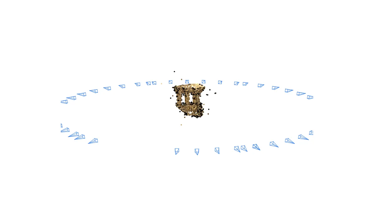
TL;DR — Structure from Motion (SfM) turns a set of overlapping photos into 3-D points plus the pose of every camera, and the whole classical pipeline fits in about 800 lines of readable Python. It rests on five ideas: feature matching (SIFT with a ratio test and RANSAC), the essential matrix relating two views, triangulation for depth, PnP to add each new view, and bundle adjustment to refine everything at once. Built from scratch with OpenCV and SciPy, the pipeline registers 47/47 images of the Middlebury temple dataset into 7,036 points at 0.25 px mean reprojection error in 23 s. COLMAP (via pycolmap) gets 47/47 at 0.30 px on the same images. Bundle adjustment matters more than anything else in the loop: without it the error grows to 0.59 px, and the first pass alone cuts it from 0.49 px to 0.13 px.

Every photogrammetry app, every “scan this object with your phone” feature, and the camera poses behind most NeRF and Gaussian-splatting captures start with this same pipeline. In practice everyone runs COLMAP [3] for it and treats it as a black box. This post rebuilds incremental SfM from scratch on real data, then checks the numbers against COLMAP itself at the end.

You’ll want the mental model from the camera-models post: the intrinsic matrix $K$ , extrinsics $[R\,|\,t]$ , and PnP all return here, now with unknown geometry instead of a known calibration target. Last time we placed a single calibrated camera. This time nothing is known except the pixels.

The running example: the patio cam goes for a walk

In the camera-models post, a fixed patio cam watched a garden. Today we unbolt it. Bruno, a garden gnome, stands 4 m in front of the camera. We take a photo, step 1 m to the right, and take another. Same gnome, two viewpoints: the smallest possible SfM problem. Every formula below gets computed on this toy world first (same camera as before: $f = 500$ px, image 640×480, principal point $(320, 240)$ ), then on real data.

The real data is the Middlebury templeRing dataset [9]: 47 photos, 640×480, taken on a ring around a plaster model of a temple. It’s 11 MB, ships with calibrated intrinsics, and is the classic benchmark for this problem, which makes it a fair place to check our pipeline. The pipeline never reads the dataset’s ground-truth poses; it only uses the images and $K$ .

Three of the 47 input photographs of the plaster temple, seen from different points on the ring.

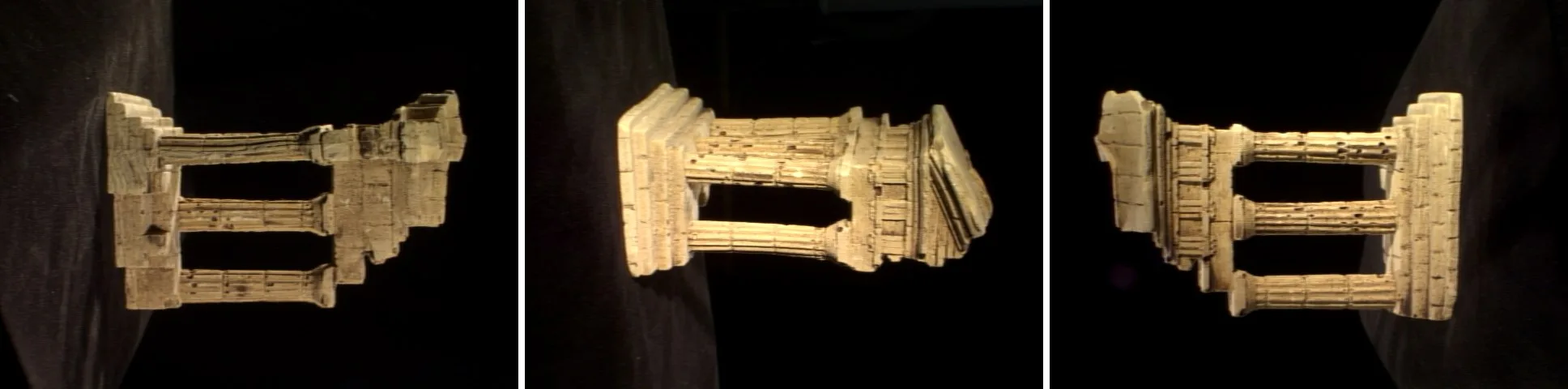
The pipeline at a glance

Incremental SfM, the strategy COLMAP made standard [3], is a loop that starts tiny and grows:

The incremental SfM pipeline with this post’s actual numbers. Everything downstream of the photos is computed; nothing else is given except K.

Each stage below gets the same treatment: the idea in plain words, the math on Bruno’s numbers, the code, and the temple results.

1. Features and matching: finding the same point twice

Reconstruction starts with one question: which pixel in photo B shows the same physical point as this pixel in photo A? Answering it robustly is what SIFT [4] is for. It detects repeatable keypoints and describes the patch around each one with a 128-number vector built to survive rotation, scale change, and lighting shifts. Szeliski covers the whole family in ch. 7 (“Feature detection and matching”) [1].

sift = cv2.SIFT_create()
keypoints, descriptors = sift.detectAndCompute(gray, None)   # ~783 kp on a temple view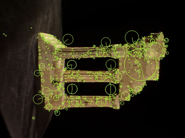

SIFT keypoints detected on one temple photograph, drawn with their detected scale.

Matching descriptors by nearest neighbour alone fails on repetitive texture (temple columns), where the nearest descriptor is often a different, identical-looking point. Lowe’s ratio test [4] keeps a match only when the best candidate is clearly better than the runner-up:

knn = cv2.BFMatcher(cv2.NORM_L2).knnMatch(desc_a, desc_b, k=2)
good = [m for m, n in knn if m.distance < 0.75 * n.distance]

The survivors look right photometrically, but some are still geometrically impossible: no rigid two-camera setup can explain them. So every pair of images gets a second filter. RANSAC fits an essential matrix (next section) and keeps only the matches consistent with it. On the temple pair below, 237 ratio-test matches become 217 RANSAC inliers; across the dataset, 237 of the 1,081 possible image pairs share enough verified matches (≥30) to enter the match graph.

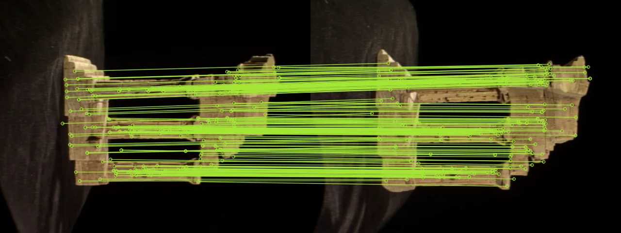
Verified matches between two temple photographs: green lines connect corresponding keypoints.

As a sanity check: neighbouring views on the ring share 200+ matches, while views from opposite sides of the temple share none, which is what you’d expect when the camera orbits an object that hides its own back side.

2. Epipolar geometry: one pixel becomes a line

A pixel $\mathbf{x}$ in image A does not tell you where the 3-D point is. It only tells you the point lies somewhere on a ray from A’s camera centre. Project that whole ray into image B and you get a line, the epipolar line, and the true match in image B must lie on it. So matching between two calibrated views is a search along a line, and choosing where on the line amounts to choosing the depth.

In symbols: for normalized coordinates $\hat{\mathbf{x}} = K^{-1}\mathbf{x}$ (pixel coordinates with the camera intrinsics undone), two views related by rotation $R$ and translation $t$ satisfy the epipolar constraint, first shown by Longuet-Higgins in 1981 along with an algorithm to recover the motion from it [6] (H&Z ch. 9, and §9.6 for E specifically [2]; Szeliski derives it in §11.3, “Two-frame structure from motion” [1]):

\hat{\mathbf{x}}'^{\,\top} E \,\hat{\mathbf{x}} = 0, \qquad E = [t]_\times R

where $[t]_\times$ is the skew-symmetric matrix that implements a cross product. Geometrically it says: the two rays and the baseline lie in one plane.

Worked example · Bruno, two photos, one metre apart

Camera A is the world origin; camera B sits 1 m to its right, not rotated. So $R = I$ and $t = (-1, 0, 0)$ (the world shifts one metre left in B’s frame), giving

E = [t]_\times R = \begin{bmatrix} 0 & 0 & 0 \\ 0 & 0 & 1 \\ 0 & -1 & 0 \end{bmatrix}.

Bruno’s nose is at $(0.5, 0, 4)$ . Its normalized coordinates: in A, $\hat{\mathbf{x}} = (0.5/4,\; 0,\; 1) = (0.125, 0, 1)$ ; in B, the nose sits at $(0.5 - 1, 0, 4)$ , so $\hat{\mathbf{x}}' = (-0.125, 0, 1)$ . Check the constraint:

E\hat{\mathbf{x}} = (0,\; 1,\; 0), \qquad \hat{\mathbf{x}}'^{\,\top} (0, 1, 0) = -0.125\cdot 0 + 0 \cdot 1 + 1 \cdot 0 = 0. \checkmark

What it means: the pair of pixels is consistent with some 3-D point under this camera motion. A mismatched pair (say, Bruno’s nose matched to his hat) would give a nonzero value, and this is the test RANSAC uses to throw out bad matches while estimating $E$ itself with cv2.findEssentialMat [10].

Now you try

Drag the point in image A and watch its epipolar line sweep image B. Every depth candidate (2 m, 3 m, 5 m, 10 m) stays glued to the line. Then shrink the baseline and watch the depth candidates bunch up: with a short baseline all depths look almost identical, which is where the triangulation problems of the next section come from.

Try it: one pixel becomes a line

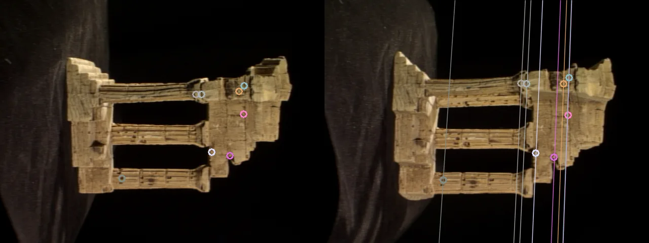
The same construction on two real temple photos: compute $E$ from the verified matches and draw the epipolar lines. Each circled point in the left image generates a line through its partner in the right image.

Epipolar lines on a real temple pair: each circled keypoint in the left image produces a colored line in the right image that passes through its matching keypoint.

3. Pose from E: four candidates, one survivor

Estimating $E$ from matches is only half the job; we still need the actual motion $(R, t)$ between the cameras. $E$ decomposes into four candidate poses (two rotations × two translation signs; Szeliski §11.3.1, “Eight, seven, and five-point algorithms” [1], and Nistér’s five-point solver [7] is the standard minimal-case method). All four explain the pixel matches equally well, but only one puts the triangulated points in front of both cameras. That test is called the cheirality check.

Decomposing E yields four (R, t) candidates. recoverPose triangulates the matches under each and keeps the only pose with the points in front of both cameras.

OpenCV handles all of it (RANSAC estimation, decomposition, cheirality test) in two calls [10]:

E, mask = cv2.findEssentialMat(pts_a, pts_b, K, method=cv2.RANSAC, threshold=1.5)
_, R, t, mask_pose = cv2.recoverPose(E, pts_a, pts_b, K, mask=mask)

Note that $\lVert t \rVert$ comes out as 1. The cameras didn’t necessarily move one metre; the equations cannot see absolute scale. We come back to this below.

4. Triangulation: where the rays cross

With both camera poses known, depth becomes computable. Each pixel back-projects to a ray, and the 3-D point sits where the two rays come closest to intersecting. The standard linear method (DLT, Direct Linear Transform) solves the small least-squares system; H&Z ch. 12 (“Structure Computation”) treats the optimal variants [2], and Szeliski summarizes in §11.2.4 (“Triangulation”) [1]. In code it’s one call [10]:

Xh = cv2.triangulatePoints(P_a, P_b, pts_a.T, pts_b.T)   # P = K [R | t]
X = (Xh[:3] / Xh[3]).T                                    # homogeneous → 3-D

Worked example · How far is Bruno's nose?

With the cameras level and parallel, triangulation collapses to the stereo disparity formula: the closer the point, the more it shifts between the photos. Bruno’s nose lands at pixel $u_A = 320 + 500 \cdot 0.125 = 382.5$ in photo A and $u_B = 320 - 500 \cdot 0.125 = 257.5$ in photo B, a disparity of $d = 125$ px. With baseline $b = 1$ m:

Z = \frac{f \cdot b}{d} = \frac{500 \cdot 1}{125} = 4 \text{ m.} \checkmark

What it means: we recovered Bruno’s true depth from pixels alone. Now add noise: ±1 px of matching error makes $d \in [124, 126]$ , so $Z \in [3.97, 4.03]$ , an answer good to ±3 cm. Shrink the baseline to 10 cm and the same point gives $d = 12.5$ px, where ±1 px yields $Z \in [3.70, 4.35]$ : around ±35 cm of uncertainty from the same pixel noise. How well depth is determined depends almost entirely on the parallax the baseline creates.

Now you try

Move the baseline, depth, and pixel-noise sliders and watch 300 noisy triangulations scatter. As the parallax angle drops, the cloud stretches along the viewing ray: depth degrades before anything else. Below about 2° the estimate is useless, which is why the pipeline drops any point triangulated with less than 1.5° of parallax.

Try it: parallax vs depth uncertainty

5. Growing the map: PnP, one photo at a time

Two views triangulate a seed cloud. Every further image is added by a loop with two steps:

Register: the new image’s keypoints match keypoints in already-registered images, and many of those already own 3-D points. That yields 2-D↔3-D correspondences, which is the input PnP needs to solve for a full camera pose (cv2.solvePnPRansac [10]).
Extend: with the new pose known, matches that don’t have a 3-D point yet get triangulated against every registered neighbour, and the cloud grows.

while (view := rec.select_next_view()) is not None:   # most 2D↔3D links first
    rec.register_view(view)          # solvePnPRansac → pose; add observations
    rec.triangulate_new(view)        # new points vs. all registered neighbours
    if len(rec.poses) % 5 == 0:
        bundle_adjust(rec)           # next section

Each new point must pass three filters, all direct consequences of the sections above: positive depth in both cameras (cheirality), reprojection error under 4 px, and triangulation angle above 1.5°.

On the temple, the pipeline picks views 32 and 47 as the seed pair (694 verified matches with 5.9° median parallax), then registers the remaining 45 images one at a time. The animation below replays that loop from the pipeline’s saved snapshots:

Close-up of the temple point cloud growing from 694 seed points to 7,036 as each of the 47 photographs is registered.

Why not just chain view-to-view relative poses (view 1 → 2 → 3 → …)? Because each essential matrix has its own unknown scale, so the chain falls apart. PnP against the shared 3-D map is what keeps every new camera in one consistent coordinate frame. The seed pair also matters disproportionately: a low-parallax seed (or one on a repeated structure) poisons every later registration, which is why the pipeline scores candidate pairs by median triangulation angle rather than match count alone.

Now you try

This lab from the camera-models post is the “register” step above: drag the pose sliders and watch reprojected points chase the observed pixels, then let Levenberg–Marquardt converge. solvePnPRansac does this for every new photo.

Try it: find the camera pose

6. Bundle adjustment: everybody moves at once

The grow loop has a flaw: every registration inherits the errors of everything before it. Pose 10 is estimated from points triangulated by poses 1–9, so errors compound. This is drift. The fix is bundle adjustment (BA): stop trusting the chain and re-optimize all poses and all points simultaneously, minimizing the total squared reprojection error (Triggs et al. is the definitive treatment [5]; Szeliski §11.4.2 [1]; H&Z §18.1 [2]):

\min_{\{R_i, t_i\},\, \{X_j\}} \;\sum_{(i,j) \in \text{obs}} \left\lVert \pi\!\left(K_i,\, R_i,\, t_i,\, X_j\right) - \mathbf{x}_{ij} \right\rVert^2

A useful mental picture: connect every camera to every point it sees with a rubber band pulling the reprojection toward the measured pixel, then let the whole structure relax at once.

Worked example · What one degree of drift costs

Suppose camera B’s estimated yaw is off by 1°. A point near the image centre reprojects roughly $f \tan(1°) = 500 \times 0.0175 \approx 8.7$ px away from its measured pixel. What it means: a pose error far too small to see in a rendering produces reprojection residuals dozens of times larger than SIFT’s sub-pixel matching accuracy. Those 8.7 px rubber bands are what BA pulls against.

At the temple’s final scale, the problem has 29,994 observations, so a residual vector of 59,988 numbers, minimized over 21,384 parameters (46 free cameras × 6 + 7,036 points × 3, with the first camera frozen to pin down the coordinate frame). Dense least-squares at that size would be hopeless, but each residual only touches one camera and one point, so the Jacobian is almost entirely zeros. scipy.optimize.least_squares exploits that sparsity [11], and each full BA pass on the temple takes about 1 s.

result = least_squares(
    residuals, x0,
    jac_sparsity=sparsity,   # each row touches 1 camera (6 cols) + 1 point (3 cols)
    method="trf", x_scale="jac", ftol=1e-4,
)

To see what BA buys, the same pipeline was run with and without it, measuring the error at every step of the reconstruction:

Mean reprojection error at each step of the temple reconstruction, from the two runs’ saved summaries (templeRing_summary.json, templeRing-noba_summary.json). The sawtooth on the blue curve: error creeps up between BA passes and each pass pulls it back down.

templeRing, 47 images	with BA (every 5 views)	without BA
images registered	47/47	47/47
3-D points	7,036	7,499
mean reprojection error	0.25 px	0.59 px
median reprojection error	0.15 px	0.27 px

Two caveats on this table. The no-BA run still finishes and still looks like a temple, because exhaustive matching plus aggressive filtering hides a lot of drift on an easy 47-image ring; on longer or harder sequences drift compounds much more severely. And the no-BA error partly stops rising because the 4 px outlier filter deletes the worst points: the error is capped by discarding evidence, not by being right. (It also ends with more points, 7,499 vs 7,036, because BA’s tightened geometry lets the filter reject more marginal points.)

The result, checked against COLMAP

The full scene, replayed from the saved snapshots — the cloud and the ring of camera poses appearing together, one photo at a time:

The reconstruction growing: a ring of 47 camera frusta appears around the temple point cloud, one photo at a time.

A GIF only shows you the orbit I chose. Here is the actual output, loaded straight from the pipeline’s saved snapshots — drag it around, and pull the step slider back to watch the 7,036 points and 47 cameras accumulate in the order the mapper created them:

Try it: orbit the temple reconstruction

Sparse cloud + camera poses drag to orbit · scroll to zoom · right-drag to pan

Loading reconstruction…

7,036 points and 47 camera frusta, 105 KiB, written by uv run sfm-webexport. Points are drawn at their final bundle-adjusted positions and revealed in creation order, so the slider shows coverage growing rather than bundle adjustment settling. The stray points floating behind the camera ring are real triangulation outliers, not rendering artefacts; the view is framed on the 1st–99th percentile so the temple is not lost among them.

As a final check, COLMAP’s own incremental mapper (via pycolmap [3]) ran on the identical 47 images:

templeRing	registered	3-D points	mean track length	mean reproj. error	wall time
mini-SfM (this post, ~800 lines)	47/47	7,036	4.3	0.25 px	23 s
pycolmap 4.1.1 (COLMAP)	47/47	7,625	6.2	0.30 px	9 s

On this small, well-behaved dataset the from-scratch pipeline holds its own: every image registered, comparable point count, comparable reprojection error. COLMAP is better everywhere engineering depth shows. It builds longer tracks (6.2 vs 4.3 observations per point, because it merges observations of the same physical point across more views instead of creating duplicates), runs 2.5× faster, and, though the table can’t show it, is far more robust on hard real-world image sets. The two reprojection errors also aren’t perfectly comparable: our pipeline uses the dataset’s known $K$ , while pycolmap self-calibrates a SIMPLE_RADIAL camera from scratch, a harder problem, which makes its 0.30 px more impressive than it looks.

The goal was never to beat COLMAP. The point is that the pipeline you can now read line by line and the one the whole field uses are built from the same five ideas [3][8].

Reproducibility

Parameter	Value
CPU	Intel Core i7-12700H (12th gen)
RAM / OS	31 GB / Ubuntu 22.04.5 LTS
Python & key versions	Python 3.12.9, opencv-python 5.0.0, scipy 1.18.0, numpy 2.5.2, pycolmap 4.1.1, rerun-sdk 0.36.0
Data	Middlebury templeRing [9]: 47 images, 640×480, 11 MB, known per-view K (ground-truth poses never used by the pipeline)
Commands	`uv run sfm-download` → `uv run sfm-run` (BA) / `uv run sfm-run --no-ba` → `uv run sfm-check` (pycolmap) → `uv run sfm-frames`
Runs	3 runs of `sfm-run`: identical reconstruction each time (47/47, 7,036 points, 0.25 px). Wall times: 23.1 s cold; 14.8–16.3 s with the cached match graph (runs 2–3 skip matching). pycolmap: single run, 9 s
Timing method	wall-clock per phase (features 1.3 s, matching 7.1 s, reconstruction+BA 14.7 s), single process, CPU only; no warmup (no GPU/JIT in the loop)
Excluded from timing	dataset download, snapshot/visualization writing
Key thresholds	Lowe ratio 0.75, RANSAC 1.5 px, PnP RANSAC 4 px, max reprojection 4 px, min triangulation angle 1.5°, BA every 5 views
Artifacts	every number above is in `output/` in the companion repo: `templeRing_summary.json` (with BA), `templeRing-noba_summary.json` (ablation), `results.md`/`results.csv` (the COLMAP comparison). `uv run sfm-viz` regenerates `templeRing.rrd`, which is the interactive replay and holds no numbers, so it is not committed

Limitations & caveats

Scale is unrecoverable. Everything is relative to the arbitrary unit $\lVert t \rVert = 1$ of the seed pair. Metric scale needs outside information.
Initialization is fragile. A low-parallax or near-pure-rotation initial pair makes $E$ degenerate. The pipeline scores seed candidates by median triangulation angle, but a scene offering no good pair (a camera that only rotates, say) has no incremental-SfM solution at all.
Repetitive structure produces ghosts. The ratio test and RANSAC reduce, but do not eliminate, wrong matches on repeated texture (identical columns, windows, tiles), and bad merges can hallucinate geometry.
These thresholds are tuned to this dataset. The 0.75 ratio, 1.5 px RANSAC and 1.5° angle work on templeRing’s clean, pre-undistorted 640×480 images. Phone photos need lens distortion handled first (what distortion does and what undistorting costs, then calibrate) and typically different thresholds.
One easy dataset, one run per configuration. The BA-vs-no-BA gap (0.59 vs 0.25 px) is measured on a single 47-image ring; treat the sizes of these numbers as illustrative rather than universal. The no-BA error is additionally capped by outlier deletion, as flagged above.
DLT triangulation is not optimal, and our BA uses plain (non-robust) least squares after filtering; industrial systems use robust losses and optimal triangulation (H&Z ch. 12 [2]).
A sparse cloud is not a surface. 7,036 points is a skeleton. Dense multi-view stereo, meshing and texturing are separate downstream stages, and the Middlebury benchmark itself [9] evaluates those.

Takeaways

SfM is five composable ideas (match, constrain with E, triangulate, register with PnP, refine with BA), and ~800 lines of Python implement all of them credibly.
A pixel in one image is a ray; seen from a second image, that ray is a line. Matching along the line and choosing the depth are the same act.
Depth accuracy is bought with parallax: the toy example that triangulates to ±3 cm at a 1 m baseline degrades to ±35 cm at 10 cm. Filter low-parallax points aggressively.
Bundle adjustment earns its cost: its first pass cut error from 0.49 to 0.13 px, and the final clouds differ by 2.4× in mean reprojection error (0.59 vs 0.25 px).
Monocular reconstruction is always up to scale; pick your unit consciously.

References

[1] Szeliski, R. (2022). Computer Vision: Algorithms and Applications (2nd ed.), ch. 7 “Feature detection and matching”, §11.2.4 “Triangulation”, §11.3 “Two-frame structure from motion”, §11.3.1 “Eight, seven, and five-point algorithms”, §11.4.2 “Bundle adjustment”, ch. 11 “Structure from motion and SLAM”. Springer. Free PDF

[2] Hartley, R., & Zisserman, A. (2004). Multiple View Geometry in Computer Vision (2nd ed.), ch. 9 “Epipolar Geometry and the Fundamental Matrix”, §9.6 “The essential matrix”, ch. 12 “Structure Computation”, §18.1 “Projective reconstruction – bundle adjustment”. Cambridge University Press. Book page

[3] Schönberger, J. L., & Frahm, J.-M. (2016). Structure-from-Motion Revisited. CVPR 2016, pp. 4104–4113. doi:10.1109/CVPR.2016.445

[4] Lowe, D. G. (2004). Distinctive Image Features from Scale-Invariant Keypoints. International Journal of Computer Vision, 60(2), 91–110. doi:10.1023/B:VISI.0000029664.99615.94

[5] Triggs, B., McLauchlan, P. F., Hartley, R. I., & Fitzgibbon, A. W. (2000). Bundle Adjustment — A Modern Synthesis. In Vision Algorithms: Theory and Practice, LNCS, Springer, pp. 298–372. doi:10.1007/3-540-44480-7_21

[6] Longuet-Higgins, H. C. (1981). A computer algorithm for reconstructing a scene from two projections. Nature, 293(5828), 133–135. doi:10.1038/293133a0

[7] Nistér, D. (2004). An efficient solution to the five-point relative pose problem. IEEE Transactions on Pattern Analysis and Machine Intelligence, 26(6), 756–770. doi:10.1109/TPAMI.2004.17

[8] Snavely, N., Seitz, S. M., & Szeliski, R. (2006). Photo Tourism: Exploring Photo Collections in 3D. ACM Transactions on Graphics, 25(3), 835–846 (SIGGRAPH 2006). doi:10.1145/1141911.1141964

[9] Seitz, S. M., Curless, B., Diebel, J., Scharstein, D., & Szeliski, R. (2006). A Comparison and Evaluation of Multi-View Stereo Reconstruction Algorithms. CVPR 2006, pp. 519–528. doi:10.1109/CVPR.2006.19 — the Middlebury multi-view datasets: vision.middlebury.edu/mview

[10] OpenCV Documentation (4.x). Camera Calibration and 3D Reconstruction (calib3d module). Docs — the code here runs on OpenCV 5.0.0, but OpenCV has not published versioned 5.x documentation at the time of writing; the calib3d functions used are unchanged between the two.

[11] SciPy Cookbook. Large-scale bundle adjustment in scipy. Tutorial

Tagged

computer-vision geometry sfm opencv fundamentals

The running example: the patio cam goes for a walk

The pipeline at a glance

1. Features and matching: finding the same point twice

2. Epipolar geometry: one pixel becomes a line

Now you try

3. Pose from E: four candidates, one survivor

4. Triangulation: where the rays cross

Now you try

5. Growing the map: PnP, one photo at a time

Now you try

6. Bundle adjustment: everybody moves at once

The result, checked against COLMAP

Reproducibility

Limitations & caveats

Takeaways

Further reading

References