What Is an Edge? Step, Ramp and Roof, and the Two Derivatives That Find Them

An edge is a place where brightness changes fast, and “fast” has a derivative in it. Worked on nine pixels by hand, the first derivative peaks at column 4 with a value of 0.30 and the second derivative is exactly 0.0000 there. Both point at the same pixel. Disturb the row by no more than 0.03 and they stop agreeing: the peak stays on column 4, while the zero-crossing slides off it.

Where we are

Lesson 1 of Edge Detection. The unit’s job is to find where one thing stops and another begins. Before any of that, we need a definition a computer can evaluate.

Take the unit’s photograph and the silhouette of a column against the black backdrop. You can point at where the column ends; a program cannot. What it can do is read one row of pixels across that boundary and do arithmetic on the numbers.

An edge is a change, and a derivative measures change

Walk across that boundary and the intensities go from dark to bright. The rate of that change is the first derivative, and on a discrete row of pixels the cheapest honest estimate is the central difference: look one step either way and halve.

$$I'[x] \;=\; \frac{I[x+1] - I[x-1]}{2}$$

Do it twice and you have the second derivative, which measures how fast the rate itself is changing:

$$I''[x] \;=\; \frac{I'[x+1] - I'[x-1]}{2}$$

The edge shows up in both, differently. Where the intensity climbs fastest, the first derivative reaches a peak. At that same place the climb stops accelerating and starts decelerating, so the second derivative passes through zero. One number to maximise, one to find a sign change in.

Not every edge is a cliff

A column against the backdrop has a sharp boundary. The border of a shadow on the base does not, and a thin highlight along a column’s edge is a third thing again. Gonzalez and Woods name the three profiles worth knowing [1]: a step, a ramp, and a roof.

The roof is the case that breaks a naive reading. If you look for a peak in the first derivative you will find two, one on each side of the ridge, and miss the ridge itself sitting between them.

Now you try

Pick a model, then widen it. Watch the first derivative of the ramp flatten into a plateau as the edge gets wider, and watch the roof produce two zero-crossings where the step produces one.

Then turn up the noise with smoothing still at zero, and read the crossing counter.

In the wild

The profiles above are drawn. Here is what an edge in a photograph actually measures.

Taking 400 rows at random from a temple cloister, finding the steepest transition in each, and measuring its equivalent width — the total rise divided by the steepest slope across it, which for a blurred step comes out at about 2.5σ and, unlike counting pixels between two thresholds, cannot be capped by the window it was measured in:

edges measured	400
median width	2.30 px
10th–90th percentile	2.11 – 2.80 px
wider than 2 px	98.8%
implied Gaussian σ	0.92 px

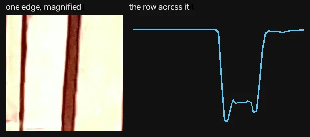
What it means: not one edge in this photograph is a step. The median transition takes 2.3 pixels and 98.8% take more than two, which is the ramp model from earlier in this lesson rather than the step model, and it is not a defect. Lenses have a point-spread function, sensors integrate over a photosite’s area, demosaicing interpolates and the anti-alias filter blurs on purpose. Every one of those widens a boundary before you see it. A detector built for perfect steps has no work to do in the real world, which is why the operators in the rest of this unit all begin by choosing a scale.

Where this breaks

Take the same nine pixels and disturb each by no more than 0.03, less than one part in thirty and invisible to the eye:

column	0	1	2	3	4	5	6	7	8
$I$	0.22	0.18	0.21	0.19	0.50	0.79	0.82	0.78	0.81
$I'$		-0.005	0.005	0.145	0.300	0.160	-0.005	-0.005
$I''$			0.075	0.1475	0.0075	-0.1525	-0.0825

The first derivative barely notices: its peak is still 0.300 at column 4. The second derivative does. It was 0.0000 at column 4 and is now 0.0075, so the sign change no longer happens at a pixel. It happens somewhere between columns 4 and 5, and the edge estimate moved half a pixel because of noise you cannot see.

That is the smaller half of the problem. On nine pixels the edge dominates the arithmetic; on a real row of several hundred, noise in the flat regions produces sign changes of its own, and a profile containing one edge reports dozens of crossings. The lab above shows it: set noise to 0.05 with smoothing at zero and read the counter.

Two consequences run through the rest of the unit. The second derivative is more fragile than the first, which is why Canny is built on the first [2] and why the zero-crossing method needs smoothing built into it rather than bolted on [3]. And even in the clean case, the ramp’s plateau means a real gradient map is thick, so something has to decide which pixel of the ridge is the edge.

Next

We have a definition and no way to apply it to an image. A row of pixels is not a photograph, and the operator has to work in two directions at once. Lesson 2 builds it, and answers why three operators that compute the same derivative behave differently on a noisy photo.

References

[1] Gonzalez, R. C., & Woods, R. E. (2018). Digital Image Processing (4th ed.), section 10.2 “Point, Line, and Edge Detection”, Edge Models, p. 772. Pearson.

[2] Canny, J. F. (1986). A Computational Approach to Edge Detection. IEEE Transactions on Pattern Analysis and Machine Intelligence, 8(6), 679-698. doi:10.1109/TPAMI.1986.4767851

[3] Marr, D., & Hildreth, E. (1980). Theory of edge detection. Proceedings of the Royal Society of London B, 207(1167), 187-217. doi:10.1098/rspb.1980.0020