Canny: Non-Maximum Suppression and Hysteresis, Taken Apart

Lesson 4 of the Edge Detection unit. Canny is two independent mechanisms, not one tuned number. NMS collapses a five-pixel ridge to one pixel by comparing along the gradient; hysteresis keeps a weak chain because it touches a strong seed. Worked on nine numbers: a single threshold gives either 1 pixel or 9, and hysteresis gives the 6 that belong to a real contour. Measured on a photo, that is 204 contours averaging 18.68 px against 393 averaging 9.69 px at the same pixel budget.

Luis Condados · August 18, 2026

computer-vision image-processing edge-detection canny fundamentals

The pipeline, one panel per stage: the photograph, its gradient magnitude, the ridge after non-maximum suppression, and what survives hysteresis.

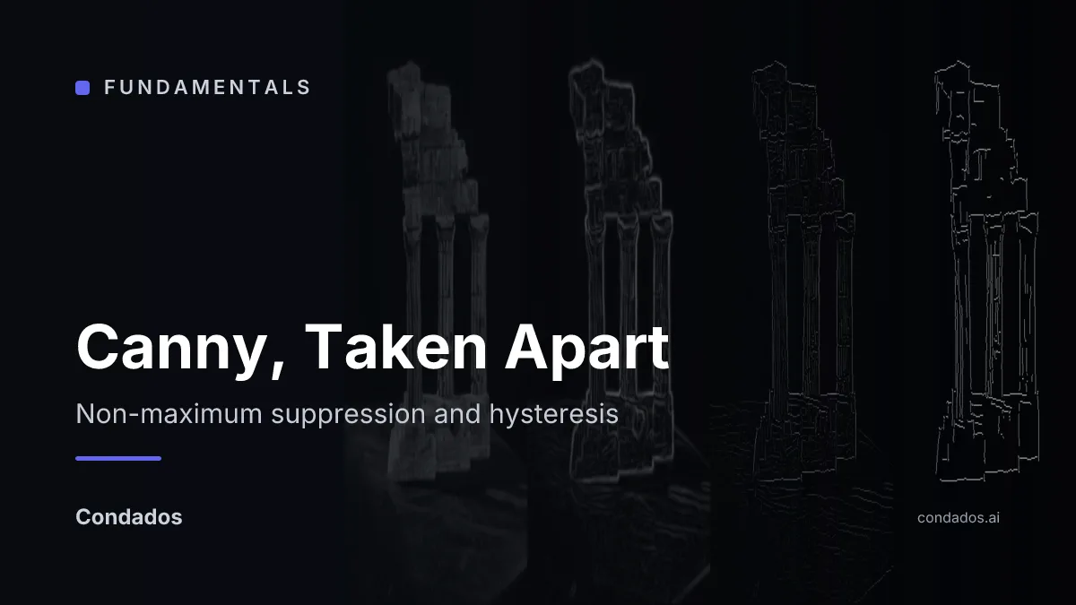
Lesson 2 left two problems that looked like one: gradient ridges come back about five pixels wide, and no single threshold gives both thin edges and full coverage. They are independent, and Canny fixed them independently. Non-maximum suppression collapses a five-pixel ridge to one pixel without consulting any threshold. Hysteresis then recovers weak pixels a threshold would have dropped, by asking whether they connect to a strong one. On nine hand-worked numbers a single threshold gives either 1 pixel or 9; hysteresis gives the 6 that belong to a real contour.

Where we are

Lesson 3 showed the second derivative can locate an edge to half a pixel but cannot rank one, so it cannot tell a shadow from a shadow. That rules it out as the backbone. We are back with the gradient from lesson 2, which has strength and orientation and is too thick.

Canny’s contribution was to state what a good detector must do: find every real edge, put it in the right place, and report it once. He then derived an operator from those requirements rather than tuning one [1]. Two of the three fall out as separate mechanisms.

Thin it: non-maximum suppression

A gradient ridge is thick because pixels either side of the true edge also see the brightness change. They see it slightly less strongly, though, and the direction in which the response falls off is the gradient direction, which lesson 2 already computed.

So: keep a pixel only if it is at least as large as its two neighbours along the gradient. Nothing is compared against a threshold and nothing is compared along the edge, so a long contour survives intact while its width collapses.

Non-maximum suppression is a local comparison, not a decision about whether an edge is real. It answers “which pixel of this ridge is the ridge” and leaves “is this ridge worth keeping” entirely alone. That separation is why the two mechanisms can be tuned independently.

Link it: hysteresis

Thinning does nothing about coverage. That is the second mechanism, and it changes the question being asked. Instead of “is this pixel strong enough”, hysteresis asks “is this pixel connected to one that is”. That is a property of a chain rather than of a pixel, and it is why no single number can express it. Two thresholds: anything above $T_{high}$ is an edge outright and seeds a chain, anything above $T_{low}$ joins a chain it touches, and anything else is dropped. Gonzalez and Woods file it under edge linking for that reason [2].

Worked example · One ridge across a column edge, then two contours

Thinning. Five gradient magnitudes across a column silhouette, on the 0 to 255 scale. The gradient points horizontally, so each pixel is compared with its left and right neighbours:

position	0	1	2	3	4
magnitude	40	120	180	110	30

Position 1: neighbours 40 and 180. Since $120 < 180$ , suppressed.
Position 2: neighbours 120 and 110. Since $180 \geq 120$ and $180 \geq 110$ , kept.
Position 3: neighbours 180 and 30. Since $110 < 180$ , suppressed.

A ridge five pixels wide becomes one pixel. Lesson 2 measured that width on the real frame at 5.10 px, and no threshold was consulted to fix it.

Linking. Now two separate thinned contours, with $T_{low} = 50$ and $T_{high} = 150$ :

contour A	60	95	170	88	62	55
contour B	70	65	58

Contour A contains 170, which is above $T_{high}$ , so it seeds. Every other pixel in A is above $T_{low}$ and connected to that seed, so the whole chain is kept: 6 pixels. Contour B has no pixel above $T_{high}$ at all. Nothing seeds it, so it is dropped entirely, all 3 pixels.

Compare against the two things a single threshold can do:

rule	pixels kept
threshold at 150	1
threshold at 50	9
hysteresis (50, 150)	6

What it means: at 150 you keep one pixel of a six-pixel contour, which is the coverage collapse lesson 2 measured. At 50 you keep contour B as well, which is the noise you were trying to exclude. Hysteresis keeps the contour that has evidence somewhere along it, and no threshold value can express that, because the rule is not about a pixel’s own value.

Now you try

The pipeline on the canonical frame, with all three parameters live. Two things to do deliberately:

Set $T_{low} = T_{high}$ . That turns hysteresis off, and the edge count drops to whatever the single threshold keeps, which the third readout shows directly. Then pull $T_{low}$ back down and watch contours grow back from their seeds.

Then raise $T_{high}$ alone. Whole contours vanish at once rather than thinning, because you are removing the seeds a chain needs, not the chain.

What it buys, measured

On the canonical frame, comparing hysteresis against a single threshold tuned to keep the same number of edge pixels, so the comparison is not just “one keeps more”:

$(T_{low}, T_{high})$	edge px	hysteresis: contours / mean length	single threshold: contours / mean length
(50, 150)	3,810	204 / 18.68 px	393 / 9.69 px
(75, 200)	2,426	109 / 22.26 px	220 / 11.03 px
(100, 250)	1,509	67 / 22.52 px	134 / 11.26 px

At an identical pixel budget, hysteresis returns about half as many contours, each about twice as long. The pixels it spends are spent on continuing contours that already have evidence, instead of on isolated fragments scattered across the frame.

How close is this to OpenCV?

The implementation here is written to be read, so it is worth asking what it agrees with. Reported per stage, because the stages do not agree equally:

stage	this implementation	OpenCV
gradient magnitude scale	—	—	median ratio 1.0001
pixels surviving NMS	32,593	32,819	0.7% apart
weak set at $T_{low} = 50$	8,403	9,810	17% apart
final edge pixels	3,810	5,564	IoU 0.573

The gradient and the thinning agree. What happens after the threshold does not, and I have not explained why. Ruled out so far: the gradient norm (OpenCV defaults to $|G_x| + |G_y|$ and is forced to the Euclidean one here), the missing blur (OpenCV applies none of its own, so the caller must), 8-bit quantization of the input, and the magnitude scale. Feeding this pipeline the quantized image moves the final count from 3,810 to 3,715, which is not the gap.

Treat the code here as a teaching implementation, not a drop-in replacement for cv2.Canny [3]. Comparing the first two rows is what tells you the mechanism is right; the last row is an open question, and reporting it as “IoU 0.573, close enough” would be the dishonest reading.

In the wild

Hysteresis is the part of Canny that is hardest to argue for in the abstract, and easiest to show on a photograph. Same image, same low threshold; the only change is whether a high threshold seeds the contours.

	edge pixels	contours	longest	over 100 px
threshold 60 alone	427,799	73,025	3,363	700
threshold 180 alone	77,780	7,258	2,173	173
60 and 180 together	170,420	4,340	3,363	654

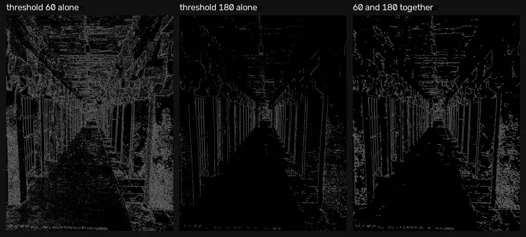
Three edge maps of the same cloister: a low threshold full of speckle, a high threshold with broken contours, and hysteresis with clean continuous lines — One low threshold, one high, and both together. The middle panel has lost the far end of the corridor; the right one keeps it without the speckle on the left. Source: “The Cloister Mandapam, in One point perspective” by Sindugab (Wikimedia Commons), CC0.

What it means, and the contour count is the number to read. The low threshold alone produces 73,025 contours to get 700 useful ones — the rest is speckle. The high threshold alone is clean but has broken the structure: 173 contours over 100 px, a quarter of what is there, because a line that dips below 180 anywhere is cut in two.

Hysteresis returns 654 long contours out of 4,340 total. It keeps 93% of what the low threshold found worth keeping while producing one seventeenth as many fragments, and its longest contour is exactly as long as the low threshold’s — the full run of the ceiling. That is the trade the second threshold buys, and no single threshold reaches it from either direction.

Where this breaks

Non-maximum suppression assumes a pixel sits on a ridge with a direction. At a junction it does not. Where a column meets the base, two edges cross and the gradient direction is whatever the stronger one happens to be, so the comparison is made along the wrong axis and one of the two arms gets suppressed. Every corner on the temple is the same problem: a corner is the one place where “the gradient direction” is not a well-defined thing.

That is not a tuning failure. No value of $\sigma$ , $T_{low}$ or $T_{high}$ recovers a junction, because the mechanism asks a question the junction has no answer to.

There is a second limit, structural. Everything so far returns curves, and a curve tells you where a boundary runs without telling you where you are along it. Two photographs of the same temple give two sets of contours with no way to say which point on one corresponds to which point on the other.

Both limits have the same fix, and it is the last lesson of the unit. Instead of asking whether brightness changes across one direction, ask whether it changes across both. That is false along an edge, true at a junction, and it gives back a point rather than a curve. Lesson 5 builds it [4].

References

[1] Canny, J. F. (1986). A Computational Approach to Edge Detection. IEEE Transactions on Pattern Analysis and Machine Intelligence, 8(6), 679-698. doi:10.1109/TPAMI.1986.4767851

[2] Gonzalez, R. C., & Woods, R. E. (2018). Digital Image Processing (4th ed.), section 10.2 “Point, Line, and Edge Detection”, The Canny Edge Detector, p. 791, and Linking Edge Points — Local Processing, p. 797. Pearson.

[3] OpenCV Documentation (5.0). Image Processing — Canny Edge Detector. docs.opencv.org/5.0

[4] Harris, C. G., & Stephens, M. (1988). A Combined Corner and Edge Detector. Proceedings of the Alvey Vision Conference 1988, pp. 1-6. doi:10.5244/C.2.23

Tagged