The Camera Response Curve: Why Your JPEG Is Not Proportional to Light

The numbers in a JPEG are not proportional to the light that made them: the camera bends them through a curve on the way to the file. Below, one exposure eases from the raw numbers, which are proportional to light, to the developed picture, with the curve drawn in the corner.

You meet this curve whenever a photo becomes a file:

• RAW versus JPEG in a camera’s or phone’s pro mode is the choice between the two ends of this animation.
• “Log” video profiles use a different curve to keep more of the scene’s range.
• Measuring anything from a JPEG (a brightness, a colour) has to undo this curve first.

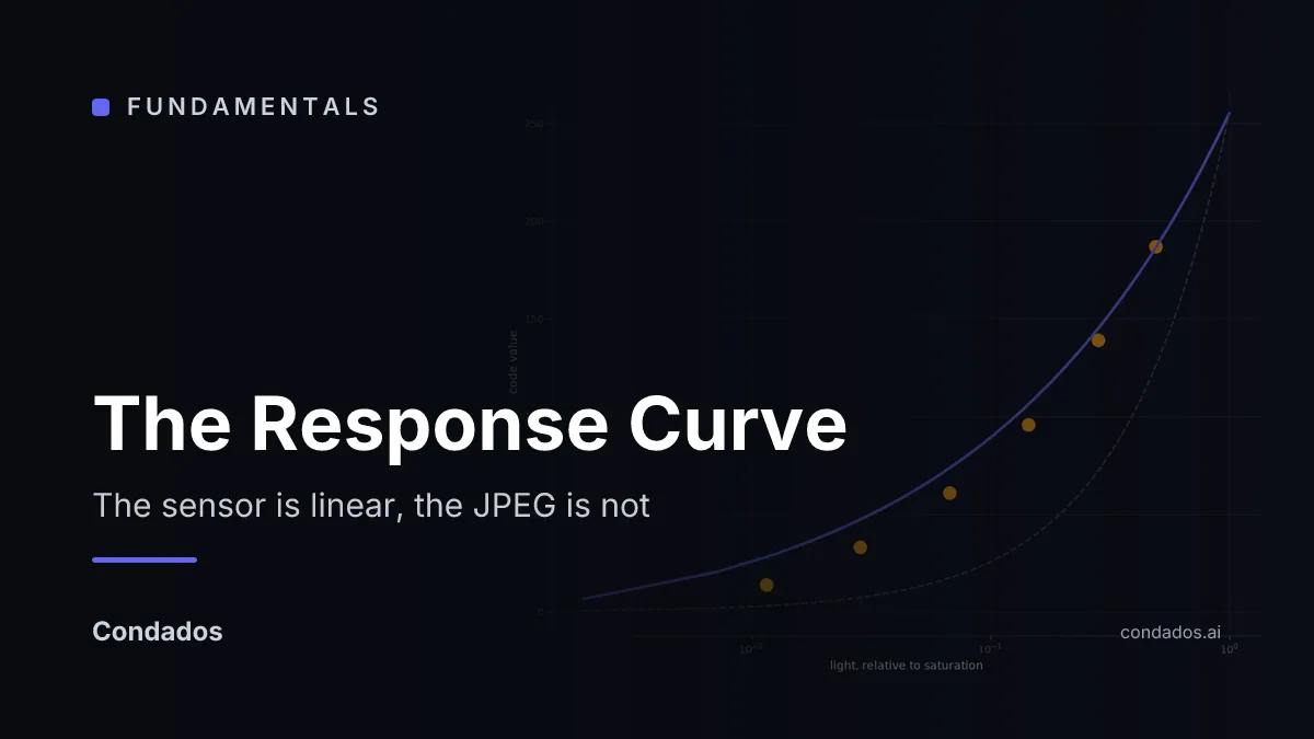
Between the sensor and the file you open sits a curve. It exists because a display is not a sensor and an eye is not a photometer, and it means the number in a developed image is not proportional to the light that made it. On the neutral ramp of this unit’s scene, six patches spanning a 42:1 range of light come out as code values from 187 to 14, a 13:1 range. The standard sRGB curve misses them by a mean of 9.6 code values; the BT.709 curve the raw developer applied by default misses by 4.0.

Where we are

Lesson 3 of image sensing. Lesson 1 established that a raw count is proportional to light, and lesson 2 measured what that count is made of. This lesson looks at the same six patches twice: once in the raw file, once in an ordinary development of it.

Why the curve exists at all

Cut a display’s brightness in half and it does not look half as bright. Human lightness perception is closer to a cube root of luminance than to luminance itself, so an image encoded in proportion to light spends most of its code values where the eye can barely tell them apart, and almost none in the shadows where it can. Store a linear ramp in 8 bits and the bottom stop of the range gets one code value out of 256; the eye wants something like a fifth of the range there. What too few code values per stop looks like is banding.

Gonzalez and Woods call the fix a power-law, or gamma, transformation [4]; encoding standards build one into the format. sRGB, which is what most files you meet are in, is close to a power law with exponent 2.2, with a short linear piece near black:

$L$ is light relative to the maximum the encoding represents and $V$ is what gets stored. sRGB is not the only such curve. Video’s BT.709 has the same shape with different constants, $V = 4.5L$ below $L = 0.018$ and $1.099\,L^{0.45} - 0.099$ above it, and it matters here because it is the curve the development below uses. Camera JPEG engines usually stack their own contrast curve on top of either. The result is a file that shows the scene well and describes it badly.

Measuring what the camera did

The scene’s lit ColorChecker has a neutral row: six patches, white through black. In raw they are counts. Developed to 8 bits by LibRaw with its defaults and no auto-brightening, they are code values. Those defaults are sRGB primaries and the BT.709 transfer curve: rawpy’s gamma parameter, left unset, is LibRaw’s $(1/2.222,\ 4.5)$ [5]. Same pixels, one frame, two numbers each:

import cv2, numpy as np, rawpy

with rawpy.imread("_MDF0005.NEF") as raw:
    linear = raw.raw_image_visible.copy()                 # counts, proportional to light
    developed = raw.postprocess(use_camera_wb=True,       # what a viewer would show you
                                output_bps=8, no_auto_bright=True)

# a patch, sampled in both: the middle 40% of the square, green photosites only
counts = np.median(linear[y0:y1:2, x0+1:x1:2])
code = np.median(cv2.cvtColor(developed, cv2.COLOR_RGB2GRAY)[y0:y1, x0:x1])

// LibRaw does both halves too: unpack() gives the raw counts, dcraw_process()
// applies the same development the Python above asks rawpy for.
LibRaw raw;
raw.open_file("_MDF0005.NEF");
raw.unpack();                                  // imgdata.rawdata.raw_image: counts
raw.imgdata.params.no_auto_bright = 1;
raw.imgdata.params.output_bps = 8;
raw.dcraw_process();                           // the developed, curve-encoded image
libraw_processed_image_t *out = raw.dcraw_make_mem_image();

What this breaks downstream

An algorithm that assumes brightness is proportional to light is relying on the dashed line and being handed the curve. Three common cases:

• HDR merging. Combining exposures means dividing each by its exposure time, and that only works on values proportional to light. Recovering the curve first is what Debevec and Malik’s method is for [1]: necessary when all you have is JPEGs, and unnecessary when you have raw, which is why lesson 4 skips it. Mitsunaga and Nayar showed the curve can be recovered from the exposures alone, without knowing the ratios exactly [2].
• Photometric methods. Shape from shading and photometric stereo solve for surface orientation from measured intensity. Feed them curved values and the recovered normals are wrong in a way that looks like a smooth deformation of the surface.
• Brightness constancy. Optical flow assumes a moving point keeps its intensity. Under a fixed curve that survives, but cameras change the curve with the scene: any auto-exposure or auto-contrast between frames breaks the assumption before the motion does.

The practical rule is short. If your pipeline reasons about light, work from raw or linearise first. If it reasons about appearance (a detector, a classifier, a tracker trained on ordinary photographs), the curve is part of the data those models were trained on, and removing it is the mistake.

Now you try

Drag the exponent to 1.0: the picture is what the sensor recorded, and it looks black. That is the whole reason the curve exists. Then add contrast and watch a single exponent stop describing the result.

The lab’s readout and the 9.6 code values above measure different curves. The lab fits a pure exponent, and $255\,L^{1/2.2}$ misses the six patches by a mean of 11.3; the 9.6 is the distance from the full sRGB function, drawn in blue. The two curves differ along the whole ramp: sRGB is a 2.4 power with an offset, which puts it 1 to 6 code values below a pure 2.2 on the three darkest patches, closer to the file. Its straight segment near black ends at $L = 0.0031$, well under the darkest patch at 0.0116, so it plays no part in either number.

In the wild

A photograph of a colour chart gives this lesson a version of its own measurement that needs no raw file, only the assumption everybody makes without noticing.

The chart’s bottom row steps from white to black. Read straight out of the JPEG, those six patches are 223.1, 203.5, 170.4, 121.2, 68.1, 14.6. Ask how much brighter the white patch is than the black one, and the answer depends entirely on what you think those numbers mean:

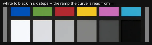
What it means: the two readings differ by 10.5×. That is the tone curve, stated as the size of the mistake rather than as a shape, and it is a mistake made constantly. Averaging code values, computing a mean brightness, blending two exposures, or measuring a reflectance ratio all assume the first column while the file was written in the second. For anything perceptual it does not matter. For anything physical, being wrong by an order of magnitude on the range of a scene is not a rounding error.

Where this breaks

• This is one converter’s idea of a good picture. The numbers above measure what LibRaw’s default development (BT.709 curve, sRGB primaries) did with this camera’s profile. Adobe’s, Nikon’s own and a phone’s all differ, and none of them publishes the curve.
• A single exponent is a description, not a model. The fit reports $\gamma = 1.47$ with $R^2 = 0.987$ and still misses the white patch by 20 code values. Quoting a gamma without the residual hides the part that matters.
• Six points is a thin ramp. The chart’s neutral row is what this scene provides; a proper characterisation walks a step wedge across the full range.
• The measurement is per channel, and colour is a further step. Neutral patches hide any difference between the red, green and blue curves. A saturated colour does not.
• Nothing here recovers the curve without raw. That is Debevec and Malik’s problem [1], and this lesson sidesteps it by having the raw file.

Next

Every count in the unit so far is a number in a file. Lesson 4 turns eighteen of them into one radiance map with a physical unit attached, and checks the result against the colorimeter readings that came with the scene [3].

References

[1] Debevec, P. E., & Malik, J. (1997). Recovering high dynamic range radiance maps from photographs. SIGGRAPH ‘97, pp. 369–378. doi:10.1145/258734.258884

[2] Mitsunaga, T., & Nayar, S. K. (1999). Radiometric self calibration. CVPR 1999, pp. 374–380. doi:10.1109/CVPR.1999.786966

[3] Fairchild, M. D. (2007). The HDR Photographic Survey. Proceedings of the IS&T 15th Color and Imaging Conference, pp. 233–238. doi:10.2352/CIC.2007.15.1.art00044. The scene and its metered points. Used for research and non-commercial publication, as its terms require.

[4] Gonzalez, R. C., & Woods, R. E. (2018). Digital Image Processing (4th ed.), ch. 3 “Intensity Transformations and Spatial Filtering”, §3.2 “Some Basic Intensity Transformation Functions”, p. 136, including “Power-Law (Gamma) Transformations”, p. 139. Pearson.

[5] LibRaw (0.22.1) and rawpy (0.27.0). Raw image decoding and postprocessing. libraw.org/docs · rawpy documentation. postprocess(no_auto_bright=True) is the development measured here; with gamma left unset, rawpy 0.27.0’s Params carries LibRaw’s default gamm = (1/2.222, 4.5), the BT.709 curve.