
What Makes a Point Matchable? SIFT, From Pixels to 128 Numbers
How SIFT turns a patch of pixels into 128 numbers that survive a moving camera. Measured on a real photo: a 45-level difference-of-Gaussians pyramid finds 791 keypoints spanning 1.8 to 112 px, each becomes a 128-dimensional descriptor, and Lowe's ratio test turns 791 candidates into 237 trustworthy matches. The invariances are real but bounded: 98.8% precision through a 45° rotation, and the scene is lost by 38° of viewpoint change. Every number has an artifact.
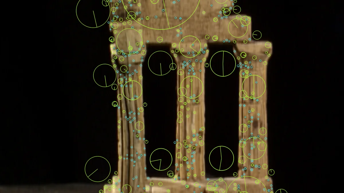
TL;DR — a point is matchable when its neighbourhood pins it down in two directions at once, and everything in SIFT follows from making that test survive changes of scale, rotation, and lighting. The test itself is the closing lesson of the Edge Detection unit; this article starts where it stops. To find such points at any size, SIFT searches a difference-of-Gaussians pyramid (45 levels for a 640×480 image) and detects 791 keypoints spanning scales from 1.8 to 112 px on our temple photo. Each keypoint becomes 128 numbers, and comparing those numbers with Lowe’s ratio test turns 791 candidate matches into 237 trustworthy ones. The invariances are real but bounded: matches survive a 45° in-plane rotation with 98.8% precision, yet fall from 406 to 21 between 8° and 38° of viewpoint change around the object.
The Structure-from-Motion post called
sift.detectAndCompute on 47 photos and moved on; the
RANSAC post cleaned up its matches.
This article opens the box those two left closed: what SIFT actually computes,
why each stage exists, and where it stops working, with every number measured on
the same temple photos [8] the other posts used. The method is Lowe’s
scale-invariant feature transform [1], and twenty years on it is still the
default front end for reconstruction pipelines.
The running example: Bruno’s hat, the wall, and the fence rail
The patio cam again. Three patches from its view of the garden:
- the blank wall behind Bruno,
- a stretch of the fence’s top rail,
- the corner of Bruno’s hat.
Suppose I cut a 21×21-pixel window around each, shuffle the photo, and ask you to find the windows again. The wall is hopeless: every candidate location looks the same. The rail is half-hopeless: you can tell you are on the rail, but any position along it matches equally well. The hat corner you can place to the pixel. Matchability is this game, and SIFT’s first job is to score it with arithmetic instead of intuition.
For real numbers we use the same photos as the SfM post: the Middlebury templeRing set [8], 640×480 images of a plaster temple on a ring of 47 camera positions. The wall, rail, and hat have stand-ins on the temple: the black background, a column’s silhouette, and the sharp corner where the base meets a column.
The test, in one paragraph
A point is matchable when its neighbourhood pins it down in two directions at once,
and that has a number attached: the two eigenvalues of the gradient structure matrix
over a window. Measured on the temple photo with a 21×21 window (artifact
output/sift_numbers.json):
| spot on the temple photo | verdict | ||
|---|---|---|---|
| background (50, 60) | 0.001 | 0.000 | flat |
| column silhouette (277, 240) | 0.411 | 0.019 | edge |
| base corner (150, 320) | 0.442 | 0.318 | corner |
Flat scores nothing in either direction, an edge scores in one, a corner in both. The derivation, the toy patches worked by hand, and a drag-the-window lab live in Corners: the structure tensor, the last lesson of the Edge Detection unit. Everything below takes that test as given and asks what has to change for it to survive a camera that moves.
The scale problem, and the pyramid that solves it
The structure matrix has a blind spot: the window size is fixed. Bruno’s hat corner fills a 21×21 window when the patio cam sees him at 3 m; walk the camera to 1 m and the same corner spans 60 pixels, so the window now sees a smooth curve and calls it an edge. A detector tied to one window size only finds features of one size.
SIFT’s answer [1] is to look for features at every size at once. Blur the image with Gaussians of increasing , stack the results, and subtract adjacent levels. Each difference-of-Gaussians (DoG) level responds to blobs and corners near one particular scale, and a keypoint is any point that is a local extremum against its 26 neighbours: 8 around it in its own level, plus 9 below and 9 above in scale.
Doubling ends an octave; the image is then halved and the ladder repeats, which is what keeps the total cost close to that of a single blur cascade.
Here is the pyramid computed on the temple photo. Reading down a column, the same subtraction is applied to an ever-smaller, ever-blurrier image, and the response moves from stone texture to whole-temple structure:
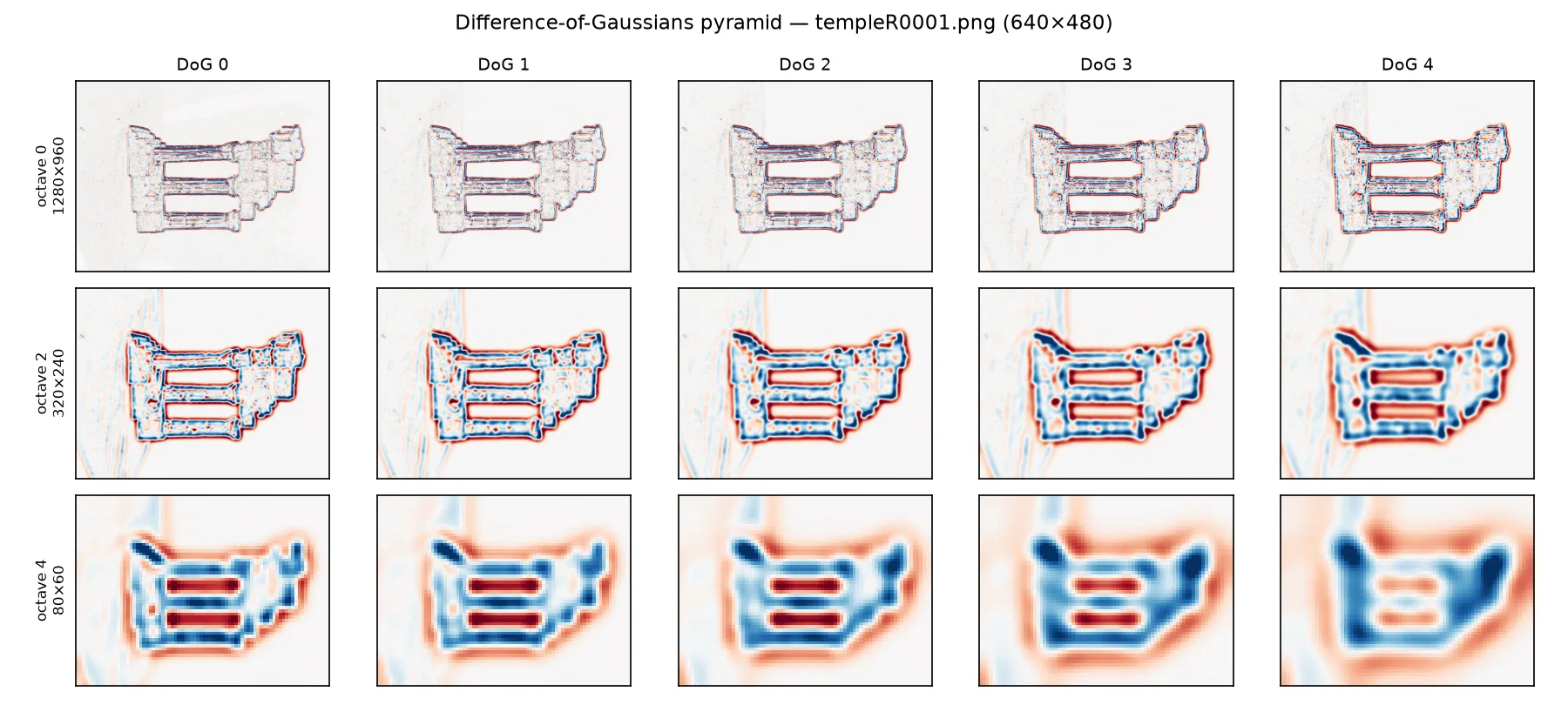
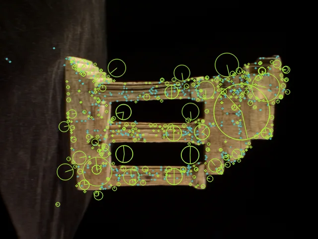
On this image, cv2.SIFT_create() detects 791 keypoints, and the detected
sizes cover almost two orders of magnitude, from 1.8 px to 112 px with a median
of 3.3 px. The octave histogram makes the pyramid’s contribution concrete: 448
of the 791 keypoints (57%) come from the upsampled octave, i.e. from structures
too small for the original resolution, and 44 come from octaves 2 and up, where
the image has been halved at least twice.
From a patch to 128 numbers
Detection answers where and at what size. Matching needs a summary of the neighbourhood that two photos can agree on, and the summary must not change when the camera rotates, zooms, or the light shifts. SIFT builds it in two steps, described in Szeliski ch. 7 [3].
Step 1: give the keypoint its own compass. Around the keypoint, at its detected scale, collect every pixel’s gradient direction into a 36-bin histogram weighted by gradient magnitude [1]. The tallest bin becomes the keypoint’s orientation, and the descriptor grid is laid out relative to it. Rotate the photo and the compass rotates along, which is where rotation invariance comes from.
Step 2: histogram the neighbourhood, coarsely. Take a 16×16 sample array around the keypoint (scaled and rotated per step 1), divide it into a 4×4 grid of cells, and build an 8-bin orientation histogram in each cell [1]:
The 128-vector is then normalized to unit length, which cancels any contrast change that multiplies all gradients equally. Values above 0.2 are clipped and the vector renormalized, so that a single glaring gradient (a specular highlight, a saturated sky edge) cannot dominate the comparison; Lowe chose the 0.2 experimentally [1]. Additive brightness shifts were already gone, because gradients ignore constants.
Matching, and the ratio test that makes it honest
Two photos, two descriptor sets. For each descriptor in photo A, find its nearest and second-nearest neighbours in photo B by Euclidean distance (Szeliski ch. 7 [3]). The nearest one is the candidate match; the second one is the honesty check. If both distances are similar, the patch has lookalikes and the match should be discarded, whatever its absolute distance. That is Lowe’s ratio test [1], and the SfM post used it as a one-liner; here it is with real numbers.
The threshold trades quantity for purity. On this pair of photos (artifact
sift_numbers.json, survivors_by_threshold):
| ratio threshold | 0.6 | 0.7 | 0.75 | 0.8 | 0.9 | 1.0 (off) |
|---|---|---|---|---|---|---|
| surviving matches | 173 | 211 | 237 | 276 | 409 | 791 |
Lowe’s experiments used 0.8, which removed 90% of false matches at a cost of under 5% of correct ones on his 40,000-keypoint database [1]; our pipeline runs 0.75. The survivors still contain geometric impossibilities (a descriptor match knows nothing about camera geometry), which is why the RANSAC post exists: on this same pair, RANSAC keeps 217 of the 237 survivors, an inlier ratio of 0.92.
In code, the whole front end is a few lines (OpenCV 5.0; the features2d
module of the 4.x line is the Features Framework in 5.0 [5]):
import cv2

sift = cv2.SIFT_create()
kp_a, desc_a = sift.detectAndCompute(img_a, None)   # 791 keypoints
kp_b, desc_b = sift.detectAndCompute(img_b, None)   # 776 keypoints

matcher = cv2.BFMatcher(cv2.NORM_L2)
knn = matcher.knnMatch(desc_a, desc_b, k=2)          # best + runner-up
good = [m for m, n in knn if m.distance < 0.75 * n.distance]  # 237 survive
#include <opencv2/opencv.hpp>
auto sift = cv::SIFT::create();
std::vector<cv::KeyPoint> kpA, kpB;
cv::Mat descA, descB;
sift->detectAndCompute(imgA, cv::noArray(), kpA, descA); // 791 keypoints
sift->detectAndCompute(imgB, cv::noArray(), kpB, descB); // 776 keypoints
cv::BFMatcher matcher(cv::NORM_L2);
std::vector<std::vector<cv::DMatch>> knn;
matcher.knnMatch(descA, descB, knn, 2); // best + runner-up
std::vector<cv::DMatch> good;
for (const auto& m : knn)
if (m[0].distance < 0.75f * m[1].distance) good.push_back(m[0]); // 237What SIFT survives, measured
The invariance claims can be tested directly. Transform the temple photo by a known warp, match against the original, and check each match against the ground-truth mapping (correct = within 3 px). No RANSAC involved; this isolates the detector and descriptor:
| transform | keypoints (791 before) | ratio-test matches | correct (≤ 3 px) | precision |
|---|---|---|---|---|
| rotate 45° | 747 | 588 | 581 | 0.988 |
| scale × 0.5 | 332 | 276 | 255 | 0.924 |
| darken × 0.4 | 165 | 174 | 159 | 0.914 |
Rotation is nearly free, as the orientation compass promised. Halving the image still matches 276 patches across a full octave of scale change. The darkening row carries the honest surprise: the descriptor held up (91% of matches correct), but the detector lost 79% of its keypoints (791 → 165), because detection applies an absolute contrast threshold that dim images fail. Invariance to illumination is a property of the descriptor, and only partially of the detector. (One knn artifact worth knowing: 174 matches from 165 keypoints is possible because two query descriptors may pick the same partner; the ratio test is not one-to-one.)
Viewpoint is the boundary that matters in practice, because walking around an object is what changes appearance in ways no 2-D warp can model. Matching temple photo 1 against photos 2 through 13, at roughly 7.7° of ring rotation per step:
| separation | 7.7° | 15.3° | 23.0° | 30.6° | 38.3° | 46.0° | 91.9° |
|---|---|---|---|---|---|---|---|
| ratio-test matches | 406 | 237 | 149 | 98 | 21 | 23 | 23 |
| RANSAC inliers | 391 | 217 | 125 | 70 | 9 | 10 | 10 |
Between 30.6° and 38.3° the pair stops being usable: 70 verified inliers is a solid relative pose, 9 “inliers” out of 21 ambiguous matches is consensus on noise. This measured cliff agrees with the standard guidance. Lowe recommends capturing training views at least every 30° of viewpoint rotation [1], and the descriptor-evaluation literature reports the same degradation pattern across all local descriptors of this family, with SIFT-like histograms merely degrading slowest [4]. It also explains a number from the SfM post: of the 1081 possible photo pairs, only 237 made it into the match graph, essentially the ring neighbours within a few steps of each other.
For a planar surface viewed obliquely, SIFT lasts longer (Lowe reports useful matching out to roughly 50° of plane tilt [1]); the temple is worse because it is a 3-D object whose columns occlude each other, so the pixels themselves change, not only their arrangement.
The neighbours
Two directions the field went from here, both worth their own article:
- ORB [6] replaces the DoG detector with FAST and the 128-float descriptor with a 256-bit binary string, matched by Hamming distance. It gives up some viewpoint and scale robustness for a couple of orders of magnitude in speed, which is why real-time SLAM systems adopted it.
- Learned features such as SuperPoint [7] train a network to output both the detector heatmap and the descriptors, with the training objective standing in for the hand-designed invariances. The classical-vs-learned matching comparison is on this site’s roadmap.
Reproducibility
| Parameter | Value |
|---|---|
| Hardware | Intel i7-12700H, 31 GB RAM (CPU only) |
| OS | Ubuntu 22.04.5 LTS |
| Versions | Python 3.12.9, opencv-python 5.0.0, numpy 2.5.2 |
| Data | Middlebury templeRing [8], views templeR0001–templeR0013, 640×480 |
| Command | uv run sfm-sift-figures in the companion repo |
| Determinism | SIFT detection and knn matching are deterministic; the RANSAC counts came out identical across 2 repeated runs |
| Artifact | every number in this post is in output/sift_numbers.json or the tables above |
| Lab photo | templeR0001 rotated upright, CLAHE contrast lift (clip 2.0, 8×8 tiles), resized to 360×480; preset eigenvalues computed on that processed image |
Limitations & caveats
- One scene, one material. Every number here comes from photos of one plaster temple. The viewpoint cliff in particular depends on geometry and texture; a flat mural would last far past 38°, a glass building would fail sooner. Treat the shape of the curve as the lesson, not the exact degrees.
- Ring separation approximates viewpoint angle. The 7.66° step assumes the 47 cameras are evenly spaced on the ring; the dataset’s calibration file shows they nearly are, but each step also changes the baseline, so “38°” bundles rotation and translation together.
- The λ thresholds in the lab are for teaching. The flat/edge/corner verdict uses a fixed cutoff (0.08 on per-pixel eigenvalues) chosen to classify this photo cleanly. Harris’s actual detector uses a smooth score and non-maximum suppression [2], and SIFT’s own edge rejection works on the DoG Hessian rather than the gradient structure matrix [1].
- The darkening result is about OpenCV’s defaults. The 791 → 165 keypoint collapse under a × 0.4 brightness cut follows from the default contrast threshold; lowering it recovers keypoints at the cost of noise. We tested one setting.
- SIFT is not fast. The SfM post measured 1.3 s of feature extraction for the 47 images (28 ms each) and 7.1 s to match all pairs, on a desktop CPU. Real-time systems pick ORB [6] or a learned detector with a GPU [7].
- A historical note: SIFT was patented by the University of British Columbia,
which is why OpenCV long kept it in
opencv_contrib; the patent has expired and SIFT now ships in the main package [5].
Takeaways
- Matchability is measurable: two eigenvalues of the gradient structure matrix separate flat (0.001/0.000), edge (0.411/0.019), and corner (0.442/0.318) on a real photo with no tuning.
- Scale invariance is bought with compute: 45 DoG levels for one 640×480 photo, and 57% of the resulting keypoints come from the upsampled octave.
- The descriptor is a rotated, normalized, deliberately coarse gradient summary; each invariance traces to one design step (compass → rotation, normalization → contrast, clipping → highlights, coarse cells → deformation).
- The ratio test needs no absolute threshold: 31.5/303.9 keeps, 349.5/349.5 rejects, and geometry (RANSAC) still has to finish the job.
- Invariance has edges: 98.8% precision under a 45° in-plane rotation, but a collapse from 406 to 21 matches by 38° of viewpoint change, which is why capture density matters more than detector choice.
Further reading
- Go deeper (the source): Lowe’s original paper [1] is unusually readable, and every design constant in this post (36 bins, 4×4×8, the 0.2 clip, the 0.8 ratio) is justified there with an experiment.
- Go deeper (the book): Szeliski ch. 7 [3] places SIFT among its alternatives and covers the matching-strategy design space our pipeline short-circuits with brute force.
- Related on CondadosAI: Structure from Motion from scratch consumes these matches to build a 3-D reconstruction · RANSAC is the geometric filter the ratio test hands over to · 2-D convolution covers the Gaussian filtering the pyramid is built from.
References
[1] Lowe, D. G. (2004). Distinctive Image Features from Scale-Invariant Keypoints. International Journal of Computer Vision, 60(2), 91–110. doi:10.1023/B:VISI.0000029664.99615.94
[2] Harris, C., & Stephens, M. (1988). A Combined Corner and Edge Detector. Proceedings of the Alvey Vision Conference 1988. doi:10.5244/C.2.23
[3] Szeliski, R. (2022). Computer Vision: Algorithms and Applications (2nd ed.), ch. 7 “Feature Detection and Matching”. Springer. Free PDF — chapter title verified against the publisher’s listing; the section numbers previously quoted here were never checked against a table of contents and have been removed rather than guessed.
[4] Mikolajczyk, K., & Schmid, C. (2005). A Performance Evaluation of Local Descriptors. IEEE Transactions on Pattern Analysis and Machine Intelligence, 27(10). doi:10.1109/TPAMI.2005.188
[5] OpenCV Documentation (5.0). Features Framework — cv::SIFT. docs.opencv.org/5.0
[6] Rublee, E., Rabaud, V., Konolige, K., & Bradski, G. (2011). ORB: An Efficient Alternative to SIFT or SURF. ICCV 2011. doi:10.1109/ICCV.2011.6126544
[7] DeTone, D., Malisiewicz, T., & Rabinovich, A. (2018). SuperPoint: Self-Supervised Interest Point Detection and Description. CVPR Workshops 2018. arXiv:1712.07629
[8] Seitz, S. M., Curless, B., Diebel, J., Scharstein, D., & Szeliski, R. (2006). A Comparison and Evaluation of Multi-View Stereo Reconstruction Algorithms. CVPR 2006, pp. 519–528. doi:10.1109/CVPR.2006.19 — the Middlebury multi-view datasets: vision.middlebury.edu/mview