Image Gradients: Central Differences, Prewitt and Sobel

A photograph has no rows and columns of interest, only pixels, so the derivative has to be measured in two directions at once and combined. On one 3x3 patch Sobel returns Gx = Gy = 1.80, a magnitude of 2.55 and an orientation of 45 degrees. Prewitt returns 1.20 and 1.70 on the identical pixels, which is why comparing operators at a shared threshold is meaningless. Across a noise sweep Prewitt recovers 0.7968 of its clean edge set at sigma = 20 against Sobel’s 0.7814, and the mechanism is one line of arithmetic.

Where we are

Lesson 1 defined an edge as a peak in the first derivative, on one row of pixels. A photograph is not one row. A column’s sides run vertically, the base runs horizontally, and the top of the temple is a staircase of both. A single row of differences finds the vertical edges and misses the horizontal ones entirely.

Two directions, then combine

Measure the derivative twice, once horizontally and once vertically, and treat the pair as a vector. Its length says how strong the change is and its direction says which way the change points:

$$|\nabla I| = \sqrt{G_x^2 + G_y^2} \qquad \theta = \arctan\!\left(\frac{G_y}{G_x}\right)$$

The gradient points across the edge, uphill toward the bright side, so the edge itself runs perpendicular to $\theta$. That perpendicular is what lesson 4 needs in order to thin a ridge, and it is carried forward again by every feature detector built on gradients [4], so orientation is not decoration here.

Measuring $G_x$ with the central difference from lesson 1 works, and it uses three pixels. The operators in practice use nine. The extra six are there to average out the rows either side of the one being differenced, and how they are averaged is the entire difference between the named operators [1]. The best known of them was never published as a paper: Sobel and Feldman presented it as a talk in 1968 and it reached print five years later, in Duda and Hart’s textbook [3].

Now you try

First the mechanics: slide the kernel one window at a time and watch the multiply-accumulate that produced the numbers above.

Then the same kernel on a real image. Switch between sobelx and sobely and notice that each is blind to edges running along its own direction, which is why you need both and then the magnitude.

Which averaging wins, measured

The three operators differ only in the smoothing vector: none, [1 1 1], [1 2 1]. Running all three on the canonical frame with noise added, at a matched budget of the strongest 5% of pixels, and asking how much of the clean-image edge set survives:

operator	sigma = 2	sigma = 5	sigma = 10	sigma = 20
central difference	0.9662	0.9158	0.8265	0.6262
Prewitt	0.9814	0.9509	0.8995	0.7968
Sobel	0.9802	0.9472	0.8948	0.7814

Averaging is worth 17 points at sigma = 20, which is the expected result. The unexpected one is that Prewitt leads Sobel at every level, by 3 to 5 times the spread across five runs, so it is not variance.

The mechanism is arithmetic rather than folklore. Noise passed through a weighted average has its variance scaled by the sum of the squared weights. Normalise each smoothing vector so it preserves brightness and compare:

$$\text{Prewitt: } \left(\tfrac{1}{3}\right)^2 \! \times 3 = \tfrac{1}{3} = 0.3333 \qquad \text{Sobel: } \left(\tfrac{1}{4}\right)^2 \!+ \left(\tfrac{1}{2}\right)^2 \!+ \left(\tfrac{1}{4}\right)^2 = \tfrac{3}{8} = 0.375$$

A box average spreads its weight evenly, and for a fixed support that is the arrangement with the smallest sum of squares. Prewitt therefore passes $0.3333 / 0.375 = 0.889$, about 11% less noise power, than Sobel. What Sobel’s [1 2 1] buys instead is a response that varies less as an edge rotates, which matters when you need the orientation and not only the magnitude.

Scope: one image, one edge budget, synthetic Gaussian noise. The ordering was consistent at every level tested, which rules out variance and does not make it a law.

In the wild

Gradients have a direction as well as a size, and on a real subject that direction is not uniformly distributed. Buildings are the clearest case: they are built plumb and level, so their edges should pile up at two orientations ninety degrees apart.

Taking the strongest 5% of gradients in the cloister and histogramming their orientation over 0–180°:

	share of strong gradients
within ±10° of the peak (0°)	53.3%
within ±10° of the perpendicular (90°)	12.2%
those two bands together	65.5%
what a uniform distribution would give	23.3%

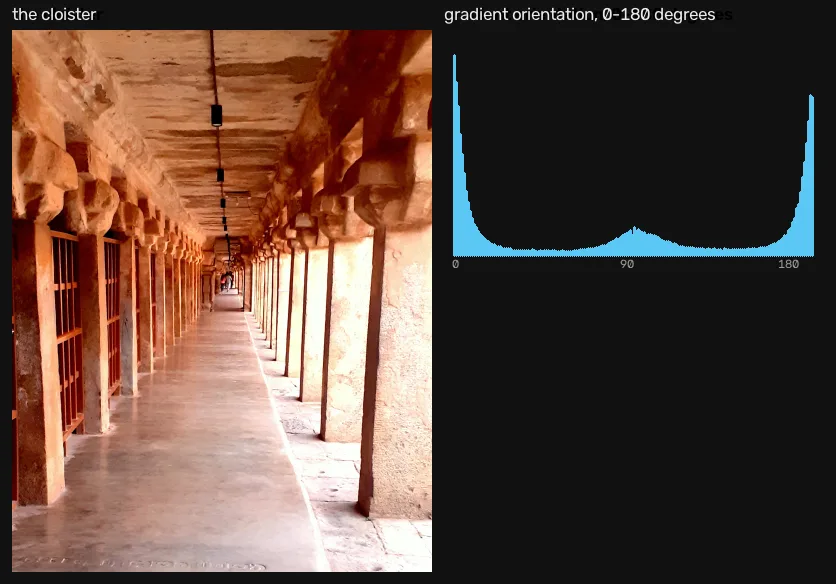
What it means: two bands covering 23% of the possible orientations carry 65.5% of the gradient energy — nearly three times what chance would give. That is the building, recovered from nothing but first derivatives. It is also the practical reason the orientation half of a gradient is worth keeping: a magnitude tells you that something changed, and it is the angle that says the change belongs to a column rather than to a shadow. Every method later in the track that bins orientations, from Hough to SIFT’s descriptor, is living on this histogram.

The asymmetry between the two peaks — 53% against 12% — is the columns being far more numerous than the horizontal beams, not the method preferring one axis.

Where this breaks

We have a magnitude per pixel. Turning that into edges means picking a threshold, and no value of it works. Sweeping the threshold on the canonical frame:

threshold	magnitude px	thinned px	ridge thickness	coverage
10	76,266	14,946	5.10 px	1.000
20	60,202	12,651	4.76 px	0.846
40	40,378	9,596	4.21 px	0.642
80	20,388	5,729	3.56 px	0.383
160	6,623	2,295	2.89 px	0.154

Ridge thickness is the magnitude pixels divided by the thinned pixels at the same threshold, so it is the average width of an edge you get back. Coverage is how much of the lowest threshold’s edge structure survives.

At threshold 10 an edge comes back 5.10 pixels wide, which is the ramp’s plateau from lesson 1 showing up in two dimensions. Raise the threshold to 160 and the ridge narrows to 2.89 pixels, but you are down to 15.4% of the edge structure. Thin and complete are not available from the same number.

One correction to the usual telling, since the sweep contradicts it: raising the threshold does not fragment the edges. The fragment count falls from 2,269 to 213 across this sweep, because weak structure disappears outright rather than breaking apart. The cost of a high threshold is coverage, not fragmentation.

Two separate problems, then. The width has nothing to do with the threshold, and the coverage has nothing to do with the width. Lesson 4 fixes them with two independent mechanisms, which is why Canny is two ideas and not one.

Next

Before that, the other derivative. The second derivative crosses zero at an edge instead of peaking, and a zero-crossing has no width to speak of, which sounds like the thickness problem solved for free. Lesson 3 takes that seriously and finds out what it costs [2].

References

[1] Gonzalez, R. C., & Woods, R. E. (2018). Digital Image Processing (4th ed.), section 10.2 “Point, Line, and Edge Detection”, Gradient Operators, p. 779. Pearson. Covers the Prewitt and Sobel masks and the magnitude/orientation definitions used here.

[2] Marr, D., & Hildreth, E. (1980). Theory of edge detection. Proceedings of the Royal Society of London B, 207(1167), 187-217. doi:10.1098/rspb.1980.0020

[3] Sobel, I., & Feldman, G. (1968). A 3x3 Isotropic Gradient Operator for Image Processing. Presented at the Stanford Artificial Intelligence Laboratory; never formally published. It first reached print in Duda, R. O., & Hart, P. E. (1973). Pattern Classification and Scene Analysis, pp. 271-272. Wiley. Sobel later published his own account as An Isotropic 3x3 Image Gradient Operator (2014). Citations of a 1968 Duda and Hart book are a conflation of the talk’s year with the book’s; the book is 1973.

[4] Szeliski, R. (2022). Computer Vision: Algorithms and Applications (2nd ed.), ch. 7 “Feature Detection and Matching”. Springer. Free PDF