
From Photons to Counts: What a Raw Number Means
A photosite collects electrons, a converter turns them into an integer, and that integer is all any algorithm ever sees. Measured on eighteen exposures of one scene: the count doubles with the shutter to within a few percent, then sticks near 3875 DN — and the ceiling the file declares is not the ceiling the sensor has.

A raw file holds one integer per photosite. That integer is a count of electrons, scaled by a gain and rounded by a converter, and it has a floor and a ceiling that belong to the sensor rather than to the picture. On the camera this unit measures, the lit chart’s white patch reads 109 DN at 1/800 s and 1902 DN at 1/45 s — five doublings of the shutter, five doublings of the count — and then it sticks near 3875 no matter how much longer the shutter stays open.
Where we are
This is lesson 1 of image sensing. The scene, the camera and the eighteen exposures come from Fairchild’s HDR Photographic Survey [3] and are introduced on the hub; this lesson only needs one fact from it, which is that the same scene was photographed at shutter speeds from 1/800 s to 30 s with nothing else changed.
A photosite is a bucket with a hole in the bottom of the scale
Light arrives at a photosite as photons. Some fraction of them free an electron in the silicon, and those electrons collect in a well until the exposure ends. Then the charge is converted to a voltage, amplified, and handed to an analog-to-digital converter that rounds it to an integer.
Write the whole chain as one line. Gonzalez and Woods call this the simple image formation model [1]; for a photosite seeing an irradiance for a time :
is how efficiently photons become electrons, is the gain in digital numbers per electron, is the black level the camera adds so noise can swing below zero without being cut off, and is the converter’s depth. Everything an algorithm ever sees has been through that line.
Three consequences fall out of it immediately, and the rest of this lesson is those three:
- The count is proportional to , so doubling the exposure doubles the count. That linearity is what lesson 4 needs to merge a bracket at all.
- The count is not electrons. It is electrons times a gain nobody wrote on the file. Until that gain is measured — which is lesson 2 — a count says how much light arrived relative to other counts, and nothing about how much light arrived.
- The well has a ceiling. Once it is full, more light changes nothing, and the number stops carrying information about the scene.
What the file says about itself
A raw file declares the sensor’s floor and ceiling. Reading them is two lines with rawpy, which wraps LibRaw [4]:
import rawpy

with rawpy.imread("_MDF0005.NEF") as raw:
    counts = raw.raw_image_visible          # one plane, still a Bayer mosaic
    print(raw.black_level_per_channel)      # [0, 0, 0, 0]
    print(raw.white_level)                  # 4095
    print(raw.camera_white_level_per_channel)  # [3827, 3827, 3827, 3827]
// LibRaw is the C++ library rawpy wraps; the same three fields live on imgdata.
#include <libraw/libraw.h>
LibRaw raw;
raw.open_file("_MDF0005.NEF");
raw.unpack();
printf("%d\n", raw.imgdata.color.black); // 0
printf("%d\n", raw.imgdata.color.maximum); // 4095
printf("%d\n", raw.imgdata.color.linear_max[0]); // 3827On this camera the black level is 0: the D2x subtracts it before writing the file. That is checkable rather than assumable — the shortest exposure in the bracket has a median of 1 DN and a minimum of 0, which is what an already-subtracted frame of a dark room looks like.
The ceiling is less tidy, and it is the first place where trusting the file costs you. Three numbers disagree:
| Source | Value |
|---|---|
white_level, as LibRaw reports it | 4095 DN |
camera_white_level_per_channel, from the file’s own tag | 3827 DN |
| Where the counts actually pile up, measured on the 30 s frame | 3880 DN (green), 4095 (red and blue) |
The two green channels stop about 200 DN below red and blue. Something in the chain treats the channels differently — the as-shot white balance this frame carries is 256 : 285 : 872 for red, green and blue, so they are certainly not equal by the time anyone looks at them — but which stage does it, and whether the greens are hitting the well or the converter, is not something these files answer. The number that matters here is the measured one: on the green channel the counts stop at 3880, and a dynamic range computed from 4095 instead is a quarter of a stop optimistic before anything else goes wrong. Deciding the mechanism would take flat fields under several illuminants, which this scene does not contain.
The count follows the exposure
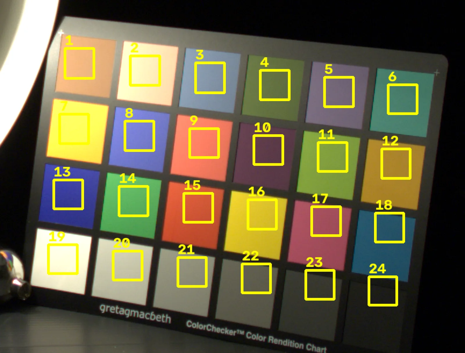
CCD or CMOS, and the part that shows up in your data
Both architectures collect charge in a well. What differs is what happens next. A CCD shifts the charge across the chip to one output amplifier, so every pixel is measured by the same electronics. A CMOS sensor puts an amplifier in each pixel and reads rows through column circuits, which is what made a camera-on-a-chip possible in the first place [2]. This sensor is CMOS, as is nearly everything you will meet.
For most work the choice is invisible. The place it becomes visible is the shutter: because a CMOS sensor is read row by row, each row starts and ends its exposure at a slightly different time unless the sensor has a global shutter. Photograph a propeller and it bends. That is not motion blur, and no denoiser fixes it — the rows are telling the truth about different instants.
What one count is, and is not
The count you read is one colour channel. A raw plane is still a mosaic: this sensor uses an RGGB Bayer layout, so the value at a given position came through a red, green or blue filter, and the other two colours at that position do not exist until demosaicing invents them. The colour filter array section of unit 1.3 covers that step; the important consequence here is that every statistic in this unit is computed on one channel at a time. Averaging a rectangle of raw pixels averages three different colours and means nothing.
Now you try
Move the light and the exposure and watch the count follow. Then raise the gain: the count follows that too, which is the reason a raw number on its own cannot tell you how much light there was.
The lab’s converter tops out at , so at 12 bits it reads 4095. That is the converter’s ceiling, not this sensor’s: the green channel of the real camera stops at 3880, for a reason the file does not record. The simulation is the ideal chain; the table above is what one camera did.
In the wild
The chart above is lit to be measured. Here is the opposite case, where almost no photons arrive at all: a long-exposure photograph of the Orion Nebula.
Most of that frame is empty sky, which makes it the honest place to ask what a count is worth. Finding the darkest, flattest 128 × 128 tile in the picture — chosen by the lowest local variance rather than by eye — gives a mean of 3.35 code values.
| background tile mean | 3.35 of 255 |
| brightest 0.01% of the frame | 255 — clipped |
| photosites at the ceiling | 1421 (0.011% of the frame) |
| photosites at the floor | 12,641 |
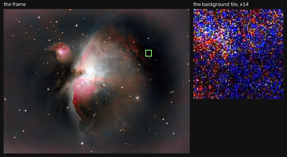
What it means: the same two limits this lesson found on the bench are both visible in one photograph, and this frame runs into both. At the top, 1421 star cores hit 255 and stopped — their real brightness is not in the file and no processing recovers it. At the bottom, 12,641 pixels sit at zero, which is the other kind of loss: not a value that was rounded, a value that was never recorded. The tile in between reads 3.35, close enough to the floor that a slightly shorter exposure would have pushed it under.
Every count between those two walls is the linear part, and it is the only part you can do arithmetic on. That is nine tenths of this frame — and it is worth knowing which tenth is not.
Where this breaks
- A count is not a measurement of light until something is measured. With gain unknown, 1902 DN is only “more than 961 and less than the ceiling”. Lesson 2 measures the gain and turns counts into electrons.
- The black level is a declaration, not a measurement. This camera writes 0 and really does subtract; others write a positive offset, and a few write one that drifts with temperature. Check it against a dark frame instead of trusting the tag.
- The ceiling is per channel. Red and blue clip at 4095 here, green at 3880, and this post does not claim to know why. Code that clips at one number for all four channels will keep saturated green pixels and throw away good red ones either way.
- Nominal shutter speeds are rounded. The exposure ratios in the worked example come out closer to 2.0 than the labelled times do. If you need exposure ratios to better than a few percent, measure them from the data rather than reading them off the EXIF.
- This is one sensor from 2004. The shape of the argument generalises; the numbers do not.
Next
The counts above were medians over hundreds of pixels, which hides the thing that makes them interesting: read the same photosite twice under identical conditions and you get two different numbers. Lesson 2 uses that spread to measure the gain, the size of the well and the range between the brightest thing the sensor can record and the faintest.
References
[1] Gonzalez, R. C., & Woods, R. E. (2018). Digital Image Processing (4th ed.), ch. 2 “Digital Image Fundamentals”, §2.3 “Image Sensing and Acquisition”, p. 41. Pearson. — the simple image formation model this lesson’s equation follows, and the sensor-array geometry behind it.
[2] Fossum, E. R. (1997). CMOS image sensors: electronic camera-on-a-chip. IEEE Transactions on Electron Devices, 44(10), 1689–1698. doi:10.1109/16.628824
[3] Fairchild, M. D. (2007). The HDR Photographic Survey. Proceedings of the IS&T 15th Color and Imaging Conference, pp. 233–238. doi:10.2352/CIC.2007.15.1.art00044 — the “Luxo Double Checker” scene and its eighteen raw exposures. Used for research and non-commercial publication, as its terms require.
[4] LibRaw (0.22.1) and rawpy (0.27.0). Raw image decoding. libraw.org/docs · rawpy documentation — raw_image_visible, black_level_per_channel, white_level and camera_white_level_per_channel are the fields quoted above.