Do it in OpenCV: M1: Fix a badly exposed photo, M2: Find every ball on a pool table

An Image Is an Array: Shape, dtype, and Why OpenCV Hands You BGR

Lesson 1 of The Image as Data. One photograph, held three ways: a 24.7 MB mosaic of 12-bit counts, a 74.2 MB 16-bit development, and the 37.1 MB 8-bit array imread would give you. Two thirds of the numbers in that last one were never measured, adding 60 to a value of 207 gives 11, and a slice you write into changes the original.

Luis Condados · August 19, 2026 · Updated September 30, 2026 · 7 min read Beginner

image-processing opencv fundamentals

Sixteen by twelve pixels of the unit's photograph, at a zoom where the numbers are legible. Source: Mark Fairchild's HDR Photographic Survey.

An image in Python is an array of numbers with a shape and a type, and the same array looks different depending on which order you read its three colour channels in. Below, one array shown with its channels in the right order and then in the wrong one.

The lamp and colour chart photograph fading between correct colours and a version where red and blue are swapped, so the orange lamp light turns blue — Nothing in the array changes, only the order in which its three channels are read. OpenCV stores blue first; most other libraries expect red first. Source: Mark Fairchild’s HDR Photographic Survey [3].

This is one of the first bugs everyone meets:

An OpenCV image shown with Matplotlib comes out with red and blue swapped, like the second half of this animation.
Faces turning blue in a video pipeline usually means one stage wrote BGR and the next read RGB.
Model inputs: a network trained on RGB and fed BGR loses accuracy without raising an error.

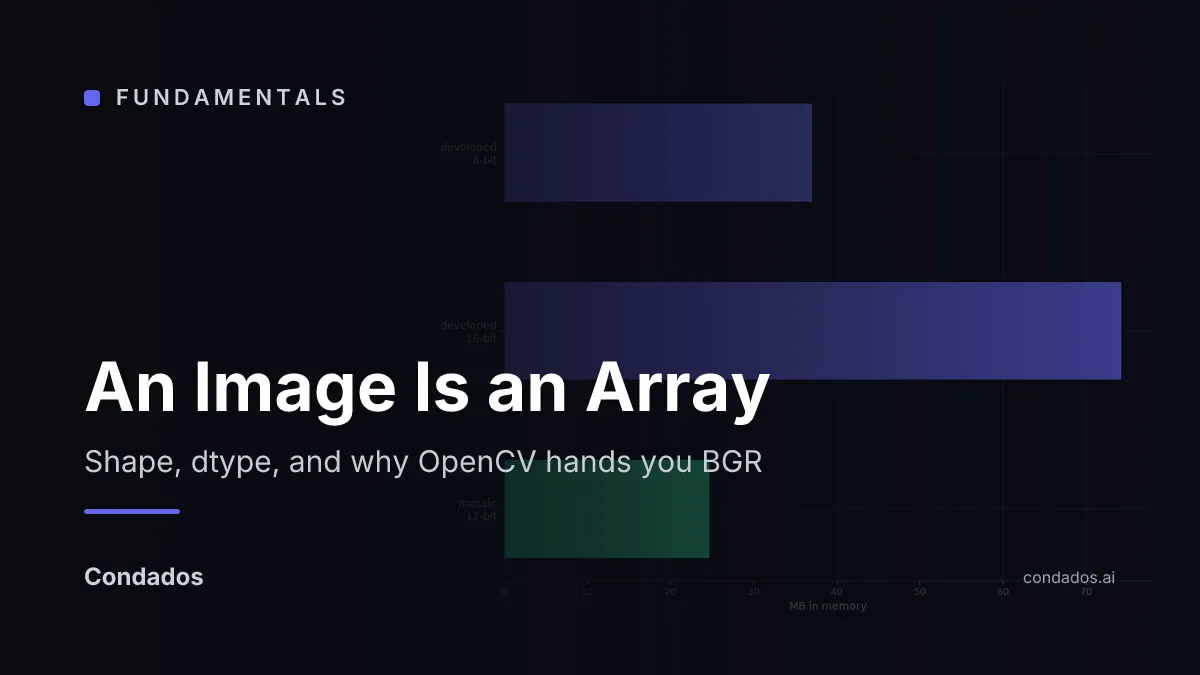
TL;DR: one photograph, held three ways: a 24.7 MB mosaic of 12-bit counts, a 74.2 MB 16-bit development, and the 37.1 MB 8-bit array imread would hand you. In that last one, two thirds of the numbers were never measured by anything; they were interpolated. Indexing is (row, column). The channels come back B, G, R. And they are 8-bit integers, so adding 60 to a value of 207 gives you 11.

Where we are

Part of The Image as Data. Unit 1.2 finished with a number in a pixel and what it counts. This lesson picks that number up and asks a duller question with a longer tail: what is the container, and what does the container do to you?

Everything below is one frame, _MDF0005.NEF (the 1/45 s exposure of the lit chart in “Luxo Double Checker”), held three different ways.

Three files, one photograph

A camera measures one number per photosite, and everything else you have ever seen from that camera is a reconstruction of the other two thirds.

	shape	dtype	in memory	at one pixel
raw mosaic	2868 × 4312	`uint16` (12 bits used)	24.7 MB	`2257`
developed, 16-bit	2868 × 4312 × 3	`uint16`	74.2 MB	`49528, 48403, 41118`
developed, 8-bit	2868 × 4312 × 3	`uint8`	37.1 MB	`193, 189, 160`

The pixel is the same place in all three rows: row 1910, column 2474, the centre of the lit chart’s white patch. The NEF on disk is 19.5 MB, which is smaller than the mosaic it decodes to, and compression is not the reason: this file’s raw data is stored uncompressed (its TIFF compression tag reads 1). The file packs each 12-bit count into 1.5 bytes, 4320 × 2868 × 1.5 = 18.6 MB of raw strips, while memory gives every count a full 2-byte uint16.

What it means: the mosaic is the only one of the three that is a measurement. It holds one number per photosite and nothing else. The other two hold three numbers per pixel, and since the sensor only ever measured one of them, two thirds of every developed image is interpolated: a number no instrument produced. Green gets half the photosites and red and blue a quarter each, which is why green survives demosaicing best (the Bayer lesson measures how much the interpolation gets wrong).

A 16 by 12 grid of large tiles, each tile one pixel of the photograph, labelled with its green channel value — Sixteen by twelve pixels of the white patch, one tile per pixel, labelled with the green value. A “flat” white patch runs from 180 to 189. The spread is the noise unit 1.2 measured, and it is why a single pixel is a poor way to ask what colour something is. Source: Mark Fairchild’s HDR Photographic Survey [3].

The array in memory

An image is stored row by row, and within a row the three channels of a pixel sit next to each other. That layout has a name, interleaved, and it is why img[100, 200] gives you three numbers rather than one.

The array is a flat run of bytes with an agreed shape on top. Row first, column second, channel last. The channel order is the one OpenCV chose, which is not the one the name RGB suggests.

Two conventions follow from that picture, and both of them bite.

Indexing is (row, column), which is (y, x). Gonzalez & Woods spend a whole subsection on this (§2.4, Linear vs. Coordinate Indexing, p. 54 [1]) because the array convention and the geometric convention disagree, and every drawing function in OpenCV takes the geometric one. img[100, 200] and cv2.circle(img, (100, 200), …) refer to two different places.

The channels come back B, G, R. imread decodes into that order and every OpenCV call assumes it [2]. In this frame, red and blue differ at 7,960,554 pixels, 64% of the image, so getting the order wrong gives a different photograph rather than a subtle tint.

import cv2

img = cv2.imread("frame.png")     # BGR, dtype uint8
print(img.shape, img.dtype)       # (2868, 4312, 3) uint8
b, g, r = img[1910, 2474]         # row first, column second
print(int(b), int(g), int(r))     # 160 189 193

#include <opencv2/opencv.hpp>

cv::Mat img = cv::imread("frame.png");        // BGR, type CV_8UC3
cv::Vec3b px = img.at<cv::Vec3b>(1910, 2474); // (row, col), BGR order
uchar b = px[0], g = px[1], r = px[2];        // 160 189 193

The numbers are integers, and integers run out

A uint8 holds 0 to 255 and nothing else, so “make it brighter” has to decide what happens at the top. NumPy and OpenCV decide differently.

Worked example · brightening the lit chart's white patch by 60

The white patch of the lit ColorChecker, sampled inside its 54 × 54 box, holds 8,748 channel values, mean 180.9, brightest 207. Add 60 to all of them.

207 + 60 = 267

267 does not fit in a byte. NumPy takes it modulo 256:

267 \bmod 256 = \mathbf{11}

OpenCV’s cv2.add clamps instead:

\min(267, 255) = \mathbf{255}

What it means: 1,579 of the 8,748 values are above 195 and therefore wrap. Under NumPy the patch mean goes from 180.9 to 194.6. It barely moves, because the brightest pixels fell to near zero and dragged the average back down. Under OpenCV it goes to 240.1. The gut check: brightening a white patch should not make it darker in places, so if you see black speckle in your highlights after an adjustment, this is what happened.

import numpy as np

patch = img[1883:1937, 2448:2502]                   # 54 x 54 x 3 = 8,748 values
brightest = patch.max()                             # 207
np.uint8(brightest) + np.uint8(60)                  # 11:  wraps
cv2.add(patch, np.full_like(patch, 60)).max()       # 255: saturates
np.clip(patch.astype(np.float32) + 60, 0, 255).max()  # 255: no surprises

# Note the trap in the obvious version: (patch + 60).max() is 255, not 11, because
# some values sat at exactly 195 and landed on the ceiling without going over it.
# The maximum of the wrapped array is not the wrap of the maximum.

// cv::Mat arithmetic saturates by default: this is cv::add's behaviour, and the
// wrap only appears if you index the buffer and do the arithmetic yourself.
cv::Mat brighter;
cv::add(patch, cv::Scalar::all(60), brighter);   // 255, clamped

uchar raw = patch.at<cv::Vec3b>(0, 0)[2];
uchar wrapped = static_cast<uchar>(raw + 60);    // 11, if raw was 207

A slice is not a copy

One more property of the container. Slicing an array gives you a view, a window onto the same memory, so writing into the slice writes into the original. Fancy indexing gives you a copy, and writing into that changes nothing.

Measured on this frame at row 1883, column 2448, the pixel reads (167, 194, 199) in imread order. Write zero into a slice of it and the original reads (0, 0, 0). Write zero into a fancy-indexed copy and the original still reads (167, 194, 199).

region = img[1883:1947, 2448:2512]
region[0:8, 0:8] = 0          # a view: img is now modified
copy = img[[1883, 1884, 1885]]
copy[:] = 0                   # a copy: img is untouched

What it means: neither behaviour is wrong, but they are opposite, and the code that mixes them up fails silently in both directions: a “non-destructive” preview that destroys the original, or a fix that never lands.

Now you try

Hover a tile to read its index and its three numbers. Then flip the channel order and watch blue and green trade places, and push the addition up with wrap on until the bright pixels go dark.

In the wild

The chart above is a bench setup. Here is the same fact on a photograph, and it is the version you will meet: a 3608 × 5509 picture of a red telephone box outside St Paul’s. On disk it is a 14.6 MB JPEG. Decoded, it is a 59.6 MB array, four times the file, because a JPEG is compressed and an array is not.

Red and blue differ at 19.8 million pixels, 99.7% of the frame. Compare that with the 64% in the lab scene above. That frame is a dark room, and in near-black pixels red and blue are both near zero, so they agree by accident. In a daylight photograph almost nothing agrees, and reading the channels in the wrong order changes the picture. The box itself, found by hue rather than by hand, has a mean BGR of (45, 40, 215). Read those same bytes as RGB and it becomes (215, 40, 45), and the mean hue of the box moves from 350°, which is red, to 242°, which is blue.

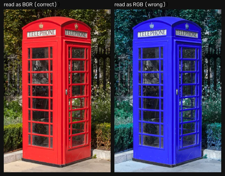
The same photograph of a red telephone box twice: correct on the left, and with red and blue exchanged on the right, turning the box blue — One array, two channel orders. Nothing was converted and no pixel moved; the same bytes were read in a different sequence. This is one of the most common bugs in the subject, and this is what it looks like. Source: “Red telephone box, St Paul’s Cathedral, London” by Christoph Braun (Wikimedia Commons), CC0.

What it means: the lab patch made the point arithmetically: 64% of pixels differ. The photograph makes it unmissable, and it shows the failure mode to expect, a scene that is confidently wrong rather than subtly tinted.

Where this breaks

The array tells you what the numbers are and nothing about where they came from. Row 1910 and row 1911 are adjacent in memory; whether they are adjacent in the scene depends on how far apart the photosites are and what fell between them. Nothing in the shape, the dtype or the channel order answers that.

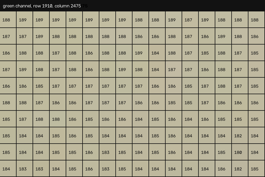
This lesson also quietly assumed that reading one pixel is a sensible thing to do. The figure above says otherwise: the “flat” white patch runs from 180 to 189. A single pixel is a sample of a noisy process, and the grid it was sampled on is the subject of the next lesson.

Sampling: what one pixel covers: the grid underneath the array, what falls between its points, and why shrinking an image the obvious way invents patterns that were never in the room.

References

[1] Gonzalez, R. C., & Woods, R. E. (2018). Digital Image Processing (4th ed.), §2.4 (Image Sampling and Quantization, p. 47), incl. Representing Digital Images (p. 49) and Linear vs. Coordinate Indexing (p. 54). Pearson. Detailed table of contents.

[2] OpenCV. cv::Mat: the basic image container and imread, OpenCV 5.0.0 documentation. Docs.

[3] Fairchild, M. D. (2007). The HDR Photographic Survey. Proceedings of the IS&T 15th Color and Imaging Conference, pp. 233–238. doi:10.2352/CIC.2007.15.1.art00044. The scene this unit measures. Used for research and non-commercial publication, as its terms require; images are downloaded, never redistributed.

Tagged