
Before this unit: Edge detection
The Hough Circle Transform: Finding Pool Balls with HoughCircles
The Hough circle transform finds round things by letting every edge pixel vote for the centres a circle through it could have. On three photos of a pool table with 41 hand-labelled balls, OpenCV's HoughCircles finds 27 with one false alarm, and 17 of 26 on the two photos it was not tuned on. Built from scratch at one radius and checked against OpenCV on the biggest ball.

The Hough circle transform finds round things in a photo, such as balls, coins and wheels, by letting every edge pixel vote for where the centre of a circle through it could be. The animation runs OpenCV’s version on the three pool-table photos this lesson measures on, then on a photo of candles: each circle appears as it is found, and the score follows.

cv2.HoughCircles (HOUGH_GRADIENT_ALT, param2=0.8). Green: a circle on a
hand-labelled ball. Amber: a circle on no ball. Pool photos by MarkBuckawicki, CC0
[4]; candles from VisA, CC BY 4.0 [5].cv2.HoughCircles, the system in the animation, step by step.- Blur the photo, so that specks and the cloth’s texture do not become edges.
- Find the edges, and for each one the direction in which its brightness changes fastest (its gradient).
- Vote. Each edge pixel votes for the points one radius away along that direction, on both sides, for every radius being searched, because the centre of a circle through it lies there.
- Find the centres. Spots where many votes pile up are candidate centres.
- Measure the radius. For each centre, the distance to its edge pixels that the most of them agree on is the radius.
You have met it in:
- Coin counters and cell counters, which find round objects of known size on a plain background.
- Eye trackers, which look for the round pupil and iris in a close-up of the eye.
- Ball tracking in sports graphics and robot football, where the ball is the one round thing on the field.
- Industrial inspection of round parts: bottle caps, drilled holes, wicks and candles.
Voting for centres finds most of the balls on a pool table with almost no false alarms, and
misses the smallest far ones and the green balls on green cloth. On three photos with 41
hand-labelled balls, OpenCV’s HoughCircles finds 27 with 1 false alarm (17 of 26 on
the two photos it was not tuned on). The colour pipeline of
OpenCV in Practice finds 29 of the same 41 with 2.
Where we are
Lesson 4, the last, of Boundary detection. Lesson 1 built the vote for lines, lesson 2 used each pixel’s gradient to vote for fewer angles, and lesson 3 fitted one line to what the vote found. This lesson runs the same pipeline for a shape with one more number. The edges come from unit 3.1’s Canny detector, and the directions from image gradients.
Naming a circle
A line needed a name of two numbers, and . A circle is every point at distance from a centre :
so its name has three numbers. The biggest ball on pool-close.webp is the circle
. Unlike slope and intercept, these three are bounded from the
start: the centre lies in the photo, and the radius in a range you choose. The cost is the third
number. A box of votes needs a cell for every centre at every radius, and one edge pixel
is consistent with every on a cone in that box. Duda and Hart wrote this down
in 1972, in the same paper that gave lines their form [2], and named the
cost: the box has to quantise the whole parameter space, so the work grows exponentially with the
number of parameters. Searched from 8 to 60 px on a 960×720 photo, it has 36,633,600 cells.
The idea: vote for the centre
Picture standing on the edge of a ball, knowing only that you are on its outline and that the ball is 52 px across the radius. The centre is 52 px away from you in some direction, so it lies on a circle of radius 52 around you. Every other pixel of the outline draws the same kind of circle, and they all cross at the true centre.
The gradient cuts that cone down. At a pixel on a circle’s outline, the gradient points along the radius, toward the centre or away from it, so at a given radius the pixel only needs to vote for two points:
where is the gradient direction. This is the same move as lesson 2, where the gradient gave instead of voting at all 180 angles; Szeliski describes it for lines and notes that the transform generalises to circles [1].
The animation below does this one radius at a time, from 12 to 56 px, on one of the photos. Each ball lights up when the radius reaches its size: the small far balls first, the big ball in front at about 52 px.

Over the whole photo at , 9,603 edge pixels cast two votes each. The best cell near the
big ball collects 14 of them. That is few, because the votes of a shaded ball scatter over a
few pixels instead of landing on one. Summing the same votes into coarser cells, which is what
HoughCircles’ dp setting does, gathers them:
| cell size | votes at the peak | peak’s distance to the label |
|---|---|---|
| 1 px | 14 | 5.1 px |
| 2 px | 36 | 5.0 px |
| 4 px | 67 | 3.6 px |
A coarser cell trades how precisely the centre is placed for how clearly the peak stands out. On this ball the coarser cells are no less accurate, because the scatter was already a few pixels wide. The animation above sums over 5 × 5 px for the same reason.
Now you try
The same photo, voting at one radius. At 52 px the big ball has the only peak over 30 votes. Move the radius down to 15 px, the size of the four far balls: one of them clears 30 votes, and so does the printed disc around the big ball’s number. Lower the votes a peak needs and watch which arrive first, balls or false circles. Then go back to 52 px and change the cell size.
How OpenCV searches every radius at once
Searching one radius at a time over the 53 radii from 8 to 60 px means a three-dimensional
accumulator of cells, and up to
votes. cv2.HoughCircles with HOUGH_GRADIENT
[3] keeps one two-dimensional accumulator of centres instead, with
cells at dp=1. Each edge pixel votes once at every radius in the
range along its gradient line, in both directions, so the votes trace two short rays and a centre
collects votes from pixels of every size of circle around it. The radius is found afterwards:
for each centre over the threshold, OpenCV looks at how far the edge pixels around it lie and
keeps the best-supported distance.
The five steps of the diagram at the top, with the settings that control each:
- Blur. A median blur removes speckle that would become short edges; the code here uses a 5 px median, as M2 did.
- Edges and gradients. Canny runs inside
HoughCircleswithparam1as its upper threshold and half of it as the lower; Sobel gives each pixel’s direction. - Vote along the gradient. Each edge pixel adds one vote at every radius from
minRadiustomaxRadius, on both sides, into one accumulator whose cells aredppixels wide. - Centres. Local maxima with more than
param2votes become candidate centres. - Radius. For each centre, the distances to the edge pixels are histogrammed and the radius
with the most support for its size kept, if that support is again over
param2. Circles closer thanminDistto a stronger one are then dropped.
HOUGH_GRADIENT_ALT follows the same plan with Scharr gradients and a different test for whether
an edge pixel supports a candidate circle: the gradient at the pixel and the line from the pixel
to the centre must point the same way, to within a cosine whose square is at least param2
[3]. At 0.8 that allows about 26.6°. The right-hand pixel of the worked example, 27.5°
off by Sobel’s measure, would fail it by about a degree.
How close is this to OpenCV?
The check: build the one-radius accumulator in NumPy on the big ball, then ask HoughCircles
where it puts the same ball. The cells fetch the photo and the hand labels that OpenCV in
Practice M2 serves [4].
import json
import numpy as np
import cv2

img = cv2.imread("pool-close.webp")
g = cv2.medianBlur(
    cv2.cvtColor(img, cv2.COLOR_BGR2GRAY), 5)
labels = json.load(open("labels.json"))
bx, by, br = max(labels["pool-close"], key=lambda b: b[2])

edges = cv2.Canny(g, 50, 150)
gx = cv2.Sobel(g, cv2.CV_32F, 1, 0)
gy = cv2.Sobel(g, cv2.CV_32F, 0, 1)
ys, xs = np.nonzero(edges)
mag = np.hypot(gx[ys, xs], gy[ys, xs]) + 1e-9
ux, uy = gx[ys, xs] / mag, gy[ys, xs] / mag

r = 52
H, W = g.shape
acc = np.zeros((H, W), np.int32)
for s in (1, -1):  # both ways along the gradient
    cx = np.rint(xs + s * r * ux).astype(int)
    cy = np.rint(ys + s * r * uy).astype(int)
    ok = (cx >= 0) & (cy >= 0) & (cx < W) & (cy < H)
    np.add.at(acc, (cy[ok], cx[ok]), 1)
print("edge pixels:", len(xs), " ball:", (bx, by, br))

for cell in (1, 2, 4):
    h, w = H // cell * cell, W // cell * cell
    a = acc[:h, :w].reshape(
        h // cell, cell, w // cell, cell).sum(axis=(1, 3))
    y0, x0 = (by - 120) // cell, (bx - 120) // cell
    win = a[y0:y0 + 240 // cell, x0:x0 + 240 // cell]
    yy, xx = np.unravel_index(win.argmax(), win.shape)
    px, py = (x0 + xx + 0.5) * cell, (y0 + yy + 0.5) * cell
    d = np.hypot(px - bx, py - by)
    print(f"cell {cell} px: {win.max()} votes"
f" at ({px}, {py}), {d:.1f} px off")edge pixels: 9603 ball: (179, 504, 52) cell 1 px: 14 votes at (183.5, 506.5), 5.1 px off cell 2 px: 36 votes at (183.0, 507.0), 5.0 px off cell 4 px: 67 votes at (182.0, 506.0), 3.6 px off
found = cv2.HoughCircles(
    g, cv2.HOUGH_GRADIENT_ALT, 1.5, 12,
    param1=300, param2=0.8,
    minRadius=8, maxRadius=60)[0]
x, y, rr = min(found,
               key=lambda c: np.hypot(c[0] - bx, c[1] - by))
print("circles on the photo:", len(found))
print(f"big ball: ({x:.1f}, {y:.1f}) radius {rr:.1f},"
f" {np.hypot(x - bx, y - by):.2f} px from the label")circles on the photo: 11 big ball: (181.5, 505.5) radius 53.3, 2.92 px from the label
OpenCV puts the big ball at (181.5, 505.5) with radius 53.3, 2.92 px from the hand label and 1.3 px larger. The one-radius NumPy accumulator puts it 3.6 to 5.1 px off, depending on the cell size. Both agree the ball is there and OpenCV is closer. I did not trace where the difference comes from; one candidate is that OpenCV estimates the radius (53.3) where the NumPy cell is given 52. I did not take the two implementations apart vote by vote, as lesson 1 did for lines: OpenCV’s two circle methods do not expose their accumulators.
Scoring it on 41 balls
M2 labelled every ball resting on the cloth in three photos of the same table by hand, as a centre
and a radius: 15 in pool, 12 in pool-close and 14 in pool-wide. A circle counts as a ball if
its centre lands within the ball’s radius (at least 8 px), one circle per ball, the same rule M2
used for its colour pipeline.
import json
import numpy as np
import cv2

labels = json.load(open("labels.json"))
grey = {n: cv2.medianBlur(cv2.cvtColor(
    cv2.imread(n + ".webp"), cv2.COLOR_BGR2GRAY), 5)
    for n in labels}

def match(found, truth):
    pairs = sorted(
        (np.hypot(x - lx, y - ly), i, j)
        for i, (lx, ly, _) in enumerate(truth)
        for j, (x, y, _) in enumerate(found))
    li, cj = set(), set()
    for d, i, j in pairs:
        if i in li or j in cj or d >= max(truth[i][2], 8):
            continue
        li.add(i)
        cj.add(j)
    return len(li), len(found) - len(cj)

def score(method, dp, p1, p2):
    hit = false = 0
    for n, truth in labels.items():
        c = cv2.HoughCircles(grey[n], method, dp, 12,
                             param1=p1, param2=p2,
                             minRadius=8, maxRadius=60)
        h, f = match([] if c is None else c[0], truth)
        hit, false = hit + h, false + f
    return hit, false

for p2 in (20, 25, 30, 35, 40):
    h, f = score(cv2.HOUGH_GRADIENT, 1, 100, p2)
    print(f"GRADIENT     param2={p2}:  {h}/41, {f} false")
for p2 in (0.7, 0.8, 0.85, 0.9):
    h, f = score(cv2.HOUGH_GRADIENT_ALT, 1.5, 300, p2)
print(f"GRADIENT_ALT param2={p2}: {h}/41, {f} false")GRADIENT param2=20: 32/41, 26 false GRADIENT param2=25: 26/41, 9 false GRADIENT param2=30: 12/41, 4 false GRADIENT param2=35: 8/41, 1 false GRADIENT param2=40: 3/41, 0 false GRADIENT_ALT param2=0.7: 28/41, 3 false GRADIENT_ALT param2=0.8: 27/41, 1 false GRADIENT_ALT param2=0.85: 23/41, 1 false GRADIENT_ALT param2=0.9: 20/41, 0 false
| method | param2 | balls found (of 41) | false alarms |
|---|---|---|---|
HOUGH_GRADIENT | 20 | 32 | 26 |
| 25 | 26 | 9 | |
| 30 | 12 | 4 | |
| 35 | 8 | 1 | |
| 40 | 3 | 0 | |
HOUGH_GRADIENT_ALT | 0.7 | 28 | 3 |
| 0.8 | 27 | 1 | |
| 0.85 | 23 | 1 | |
| 0.9 | 20 | 0 |
What it means: with HOUGH_GRADIENT, param2 is a vote count, and moving it from 20 to 30
takes the false alarms from 26 to 4 and the balls found from 32 to 12; there is no setting that
gets most balls without a crowd of false circles. HOUGH_GRADIENT_ALT’s param2 tests how well each edge
pixel’s gradient points at the centre; at 0.7 and 0.8 it finds 28 and 27 balls with 3 and 1
false alarms. The circles it finds have a median radius error of 1.3 px.
Picking the best row of a table and reporting it flatters the method, because the setting was
chosen on the same balls it is scored on. So each method’s param2 was also chosen on pool alone
(most balls found minus false alarms) and scored on the other two photos, 26 balls it never saw:
method, tuned on pool | chosen param2 | found on the other two (of 26) | false alarms |
|---|---|---|---|
HOUGH_GRADIENT | 25 | 15 | 8 |
HOUGH_GRADIENT_ALT | 0.8 | 17 | 1 |
| M2’s colour pipeline, all three photos | 29 of 41 | 2 |
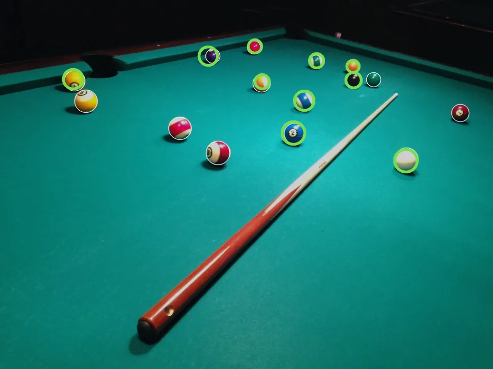
pool, the photo param2 was chosen on: HOUGH_GRADIENT_ALT at 0.8 finds 10 of 15
balls with no false alarm. White outlines with no green circle are the misses. Photo by
MarkBuckawicki, CC0 [4].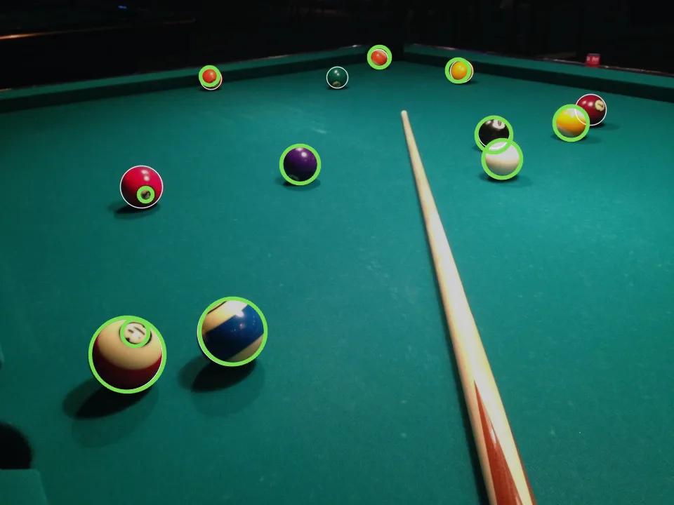
HOUGH_GRADIENT_ALT at param2=0.8 on pool-close: 10 of 12 balls. The one false
alarm is the small circle at (192, 474), radius 19, which is the white disc printed around the
big ball’s number. The red ball on the left counts as found through the same kind of mistake: the
circle on it is its number disc, radius 10.5 against the ball’s 30, and the match rule only asks
that the centre fall inside the ball. Photo by MarkBuckawicki, CC0 [4].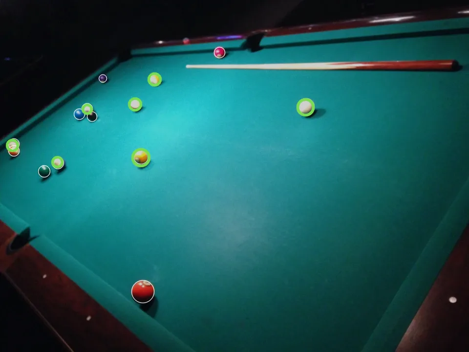
pool-wide: 7 of 14, in green; white outlines with no green circle are the misses. Six of the
seven are far balls 8 to 12 px in radius. Photo by MarkBuckawicki, CC0 [4].In the wild
A candle seen from above is a circle of known size, and a production line photographs thousands of
them. On 100 photos of the candle category of VisA, an industrial-inspection dataset whose candle photos show four
tea lights on a dark background [5], the same HOUGH_GRADIENT_ALT at param2=0.8, with
the radius range set to 40 to 200 px and minDist to 40:
| photos | 100 |
| photos with exactly 4 circles | 100 |
| radius, median | 144.4 px |
| radius, 5th to 95th percentile | 142.7 to 146.3 px |
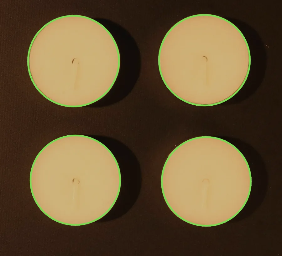
candle (Zou et al., ECCV 2022), CC BY 4.0
[5].What it means: on a controlled scene, with one size of object, a plain background and a camera that never moves, the transform returns four circles on every photo, and their 400 radii agree to within about 2 px of each other. The candles have no hand labels, so this is a count and a consistency check, not a check of each circle’s position; the photo above is typical of the 100. The pool table is the harder case, and the difference between the two is the list below.
Where this breaks
Circles that are not the object. The one false alarm on pool-close is the white disc around
the big ball’s number: a real circle, on the ball, of a size inside the search range. Any round
logo, coin-shaped highlight or pocket of the table looks the same to the vote.
Small, distant balls. At 8 to 12 px of radius, a ball’s outline is 50 to 75 pixels long, and
on the big ball above only about half of the outline turned into edge pixels. Six of the seven
balls missed on pool-wide are that small.
Green on green. Two of the misses are the green balls, one in pool and one in pool-close,
whose edge against the cloth is faint. For the other six misses, mid-sized balls in pool and
pool-close, I did not find a single cause.
The match rule is generous. A circle counts if its centre lies inside a labelled ball, so the number disc on the red ball counts as finding the red ball. Requiring the radius to agree as well would turn that one into a miss and a false alarm.
The radius range is a cost and a prior. Each extra radius adds two votes for every edge pixel, and every round thing of a size inside the range is a candidate. Knowing the size of what you are looking for, as with the candles, did most of the work there.
param2 with HOUGH_GRADIENT has no safe value. The table above goes from 26 false alarms to
1 while the balls found go from 32 to 8; a value chosen on one photo kept 8 false alarms on the
other two.
Three photos and one table. 41 balls means one ball is 2.4 percentage points, and the held-out
score is on 26. The settings for HOUGH_GRADIENT_ALT came from a sweep on these photos.
What to use it for. HOUGH_GRADIENT_ALT finds about as many balls as M2’s colour pipeline,
27 of 41 against 29, with one false alarm against two, and it needs no colour range for the cloth.
Use it when the objects are round, of a known range of sizes, and their outline shows; use colour
when the outline does not, and expect the small far ones to need a closer camera with either. I did
not check whether the two methods miss the same balls.
Exercises
- Where does one pixel vote? Write
centre(x, y, direction, r), returning the point pixels from along the gradient direction, given in degrees. Use the worked example’s pixels to test it.
import math

def centre(x, y, direction, r):
    return (x, y)  # move r pixels along the direction

print(centre(179, 454, 86.7, 52))
print(centre(216, 466, 130.0, 52))- Predict, then run. In the scoring cell,
HOUGH_GRADIENT_ALTatparam2=0.9: will it find more or fewer than 27 balls, and how many false alarms? - Break it. Run
HOUGH_GRADIENTatparam2=20, then 30. Before running, guess which gives more false alarms than balls found.
What you should see
These come from section 4 of the unit notebook, boundary_detection.ipynb, and are the same on
OpenCV 4.11 (this page) and 5.0.
(181.99…, 505.91…)and(182.57…, 505.83…), which round to (182, 506) and (183, 506).- Fewer: 20 of 41, with no false alarms.
- At 20, 32 balls and 26 false alarms; at 30, 12 balls and 4 false alarms. Neither has more false alarms than balls, but at 20 almost half the circles are wrong.
Check yourself
Four questions on this lesson. Pick an answer to see why it is right or wrong.
At a known radius r, how many centres does one edge pixel vote for when it uses its gradient?
On a circle’s outline the gradient points along the radius, toward the centre or away from it, so only two candidate centres are left at each radius.
At r = 52, the best single-pixel cell at the big ball collects only 14 votes. What does summing votes into 4 px cells do?
A shaded ball’s votes scatter over a few pixels. Coarser cells, which HoughCircles sets with dp, trade precision for a clearer peak; here the scatter was already that wide.
With HOUGH_GRADIENT, moving param2 from 20 to 30 takes the balls found from 32 to 12. What happens to the false alarms?
With HOUGH_GRADIENT, param2 is a vote count, and no value gets most balls without many false circles. HOUGH_GRADIENT_ALT at 0.7 and 0.8 finds 28 and 27 balls with 3 and 1 false alarms.
The one false alarm of HOUGH_GRADIENT_ALT on pool-close is a real circle. What is it?
It is round and of a size inside the search range, so the vote cannot tell it from a ball. The same kind of disc on the red ball is credited as finding that ball by the generous match rule.
Next
This closes the unit. Boundary detection puts the four lessons side by side, with the measurements and their limits. From here, unit 3.3 turns from shapes to points: what makes a point in one photo findable in another, starting with SIFT. The OpenCV in Practice pool table project is the same table found by colour.
Further reading
- Duda and Hart’s paper [2], the last two pages, for the circle as a cone in three dimensions and the warning about the number of parameters, in their words.
- Szeliski §7.4.2 [1], for the oriented vote this lesson borrows from lines.
- The OpenCV in Practice pool table project, for the same 41 balls found by colour, and why touching balls defeat that.
- OpenCV’s
hough.cpp[3],HoughCirclesGradientandHoughCirclesAlt, for the two-stage centre-then-radius search as code.
References
[1] Szeliski, R. (2022). Computer Vision: Algorithms and Applications (2nd ed.), §7.4.2 “Hough transforms”, pp. 477–479 (the oriented vote, Figure 7.47; footnote 15 on p. 478 on generalising to circles). Springer. Free PDF
[2] Duda, R. O., & Hart, P. E. (1972). Use of the Hough Transformation to Detect Lines and Curves in Pictures. Communications of the ACM, 15(1), 11–15. doi:10.1145/361237.361242
[3] OpenCV 4.11.0 source, modules/imgproc/src/hough.cpp: HoughCirclesGradient (line 1649; the vote along the gradient for every radius from line 1226), HoughCirclesAlt (line 1775; the test of the gradient against the line to the centre, minCos2, at line 2017) and the param2 < 1.0 check for HOUGH_GRADIENT_ALT (line 2322), commit 1d3b34d.
[4] MarkBuckawicki. Billiards table 2.JPG, Billiards table 1.JPG and Billiards Table.JPG (27 Feb 2014). Wikimedia Commons, CC0 1.0. commons.wikimedia.org

[5] Zou, Y., Jeong, J., Pemula, L., Zhang, D., & Dabeer, O. (2022). SPot-the-Difference Self-Supervised Pre-training for Anomaly Detection and Segmentation. ECCV 2022. arXiv:2207.14315 · DOI:10.1007/978-3-031-20056-4_23. Dataset CC BY 4.0.