Camera Geometry: From a 3-D Point to a Pixel, and Back to the Camera

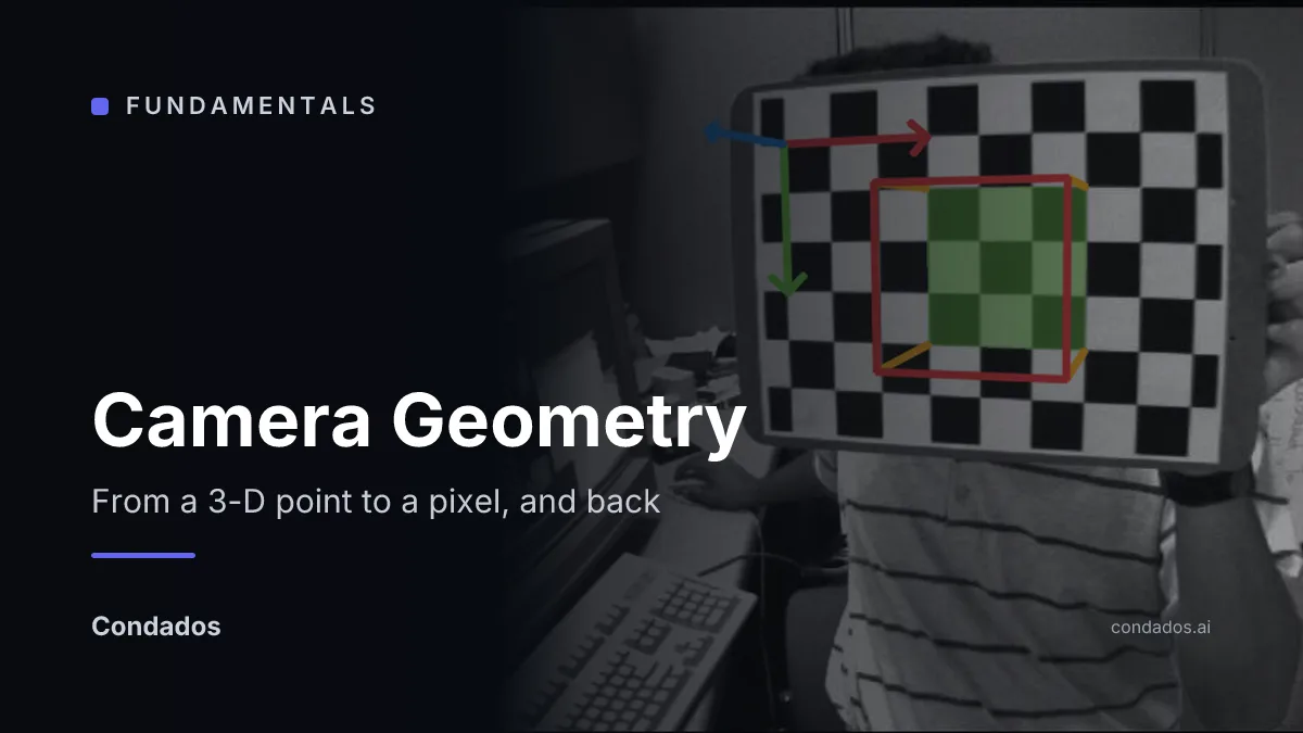
This unit is about the camera as a piece of geometry: one rule that sends any point of the world to a pixel, and that can be run backwards to find the camera itself, its focal length and where it stood. The same rule is behind every AR app, every robot that docks on a printed marker and every 3-D model built from photos. The animation shows the finished result: for each photograph of a chessboard, the board’s axes drawn from the recovered pose, and every camera position seen from above.

Every lesson is one step of the same pipeline:

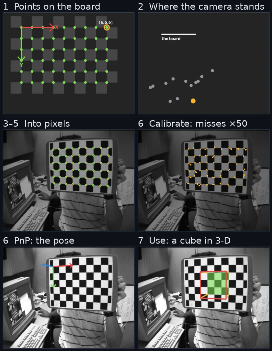
1. A point on the board. Every inner corner of the printed chessboard has a known position on it: $(8, 0, 0)$ is eight squares along the top row. The board is the world.
2. Move it into the camera’s frame. A rotation $R$ and a shift $t$ say where the camera stands relative to the board: six numbers, different for every photo (lesson 2).
3. Divide by depth. The point’s direction from the camera, which is where perspective comes from; homogeneous coordinates turn that division into one matrix product and give parallel lines somewhere to meet (lesson 1).
4. The lens bend. Real glass bends each ray a little; unit 1.1 measures and undoes it, and this unit uses its coefficients.
5. Into pixels. The focal length in pixels and the image centre, the matrix $K$: five numbers that belong to the camera and not to the photo (lesson 2).
6. Compare with what was detected. The corners found in the photo against the corners the model predicts. Many photos of the board fix $K$ and the lens: that is calibration (lesson 3). One photo with $K$ known fixes $R$ and $t$: that is PnP (lesson 4).
7. Use it. Draw something in 3-D on the board, place the camera on a map, or measure.

What the outputs are used for

Each use acts on a number this pipeline returns:

• Augmented reality on a marker. ArUco and AprilTag markers give four known corners; PnP turns them into the camera’s pose every frame, and the app draws through $K[R|t]$, as the cube in panel 6.
• Robots and drones dock on a printed pattern of known size: the pose’s distance and angle are what the controller closes the gap on.
• Measuring from a fixed camera. With $K$ and the pose of the floor known, a pixel on the floor becomes a position in metres; the homography unit is the flat case of the same idea.
• 3-D reconstruction. Structure from motion adds each new photo to its model by PnP against the points it has already built.
• Any camera used for measurement is calibrated first, and its reprojection error is the number that says whether to trust it.

A camera is one matrix that sends a point of the world to a pixel, and run backwards on an object of known shape it gives you the camera’s focal length and where it stood. Thirteen photos of a printed board calibrate OpenCV’s sample camera to 0.41 px, and when five of a photo’s corners are wrong, a robust pose moves the camera by 0.008 board squares where a plain one moves it by 2.5.

Before this

You need image formation, unit 1.1: the pinhole equations and the lens bend are its lessons, and this unit puts them into one matrix. The calibrated camera this unit uses is the same one unit 1.1 measured.

How to write down a camera

The first way to write a camera down is the one unit 1.1 used: rotate and shift the point into the camera’s frame, then two equations per pixel,

$$u = c_x + f_x\,\frac{X_c}{Z_c}, \qquad v = c_y + f_y\,\frac{Y_c}{Z_c}$$

It works for one point and one camera, and it fails at two jobs a vision pipeline does all the time:

• Composing and undoing. Rotation, shift, division and scaling are four different operations, so chaining two cameras, or solving for the camera from pixels, is a pile of special cases.
• Points at infinity. The equations take a point at a finite position, and parallel lines meet only at infinity. On the board’s first photo, the board’s rows appear to meet at a point 1,569 px left of the frame; on unit 3.5’s court the two sidelines meet 332 px past the right edge. Computing those points means pushing the place where the lines meet, at infinity, through the camera, and the two equations have no way to write that place down.

The better form writes the point as four numbers, $(X, Y, Z, 1)$, and the whole camera as one 3×4 matrix:

$$\begin{pmatrix} u\,w \\ v\,w \\ w \end{pmatrix} = \underbrace{K}_{\text{who the camera is}}\;\underbrace{[\,R \mid t\,]}_{\text{where it stands}} \begin{pmatrix} X \\ Y \\ Z \\ 1 \end{pmatrix} = P \begin{pmatrix} X \\ Y \\ Z \\ 1 \end{pmatrix}$$

On the first photo, the board corner $(8, 0, 0, 1)$ goes to $P$ times it, $(7248.74,\ 1078.25,\ 13.834)$, and dividing by the last entry gives the pixel $(523.98, 77.94)$. With unit 1.1’s lens bend added it lands at $(514.05, 86.72)$, 0.34 px from where the detector found the corner. Composing is now multiplying, and the board’s X axis at infinity is $(1, 0, 0, 0)$: it lands where the formula says, off the left edge [1] [2].

The two scenes

Lesson 1: a court. Homogeneous coordinates was written with the homography unit and runs on its pickleball frame, where a corner sits outside the photo and the sidelines meet off it.

Lessons 2 to 4: a chessboard. OpenCV’s own thirteen 640×480 photographs of a board with 9×6 inner corners (Apache-2.0), the same set unit 1.1 calibrates. Its square size is not published, so every distance here is in board squares, and no number in this unit is in metres: $K$, the lens coefficients and every pixel error are unaffected by that choice.

Topics

1. Homogeneous coordinates. Step 3 and its points at infinity: why vision adds a 1, and how the line through two points and the point where two lines cross become one cross product.
2. The camera matrix. Steps 2 to 5: $K$, $[R|t]$ and the 3×4 matrix $P$, worked on one corner of the board and taken apart again [1].
3. Calibration. Step 6 with many photos: how thirteen views of a flat board fix $K$ and the lens, and how to tell a good calibration from one that only fits its own photos [3].
4. PnP. Step 6 with one photo: where the camera stood, from points of known position, and what to do when some of them are wrong [4].

The order follows the pipeline: the representation first, then the forward camera, then the two ways of running it backwards.

What the unit measures

Every number below is a key in output/camera_geometry_numbers.json, in board squares where it is a distance.

Result	Measurement
Thirteen photos calibrate the camera	RMS 0.4087 px over 702 corners; $f_x$ 536.07, $f_y$ 536.02, centre (342.37, 235.54)
A held-out photo scores like the fitted ones	Calibrated on 12 and scored on the 13th, a median 0.204 px per view against 0.194 in-sample
Three photos are not enough	Over all 286 three-photo subsets, $f_x$ ranges from 519.6 to 567.9 (5% to 95%: 530.2 to 544.3)
The lens model is not optional	With no distortion terms the RMS is 1.555 px, and $f_x$ moves to 557.45
PnP returns the calibration’s own pose	On the first photo the two poses differ by 0.00002° and 0.00001 squares
Four corners give a usable pose	From the four outer corners, 0.269 px on all 54 and the camera 0.073 squares off
Noise moves the camera a little	1 px of noise on every corner, 200 times: a median 0.145 squares, at 16.85 squares away
Wrong corners need a robust fit	Five corners moved 25–50 px: plain PnP moves the camera 2.517 squares, RANSAC 0.0079

Limitations & caveats

• Board squares, not metres. The board’s square size is not published with these photos. Any distance here becomes metres by multiplying by the square’s size, which is a measurement this unit does not have.
• One camera. The calibration describes one 640×480 camera from OpenCV’s samples. A different camera has a different $K$; the method carries over, the numbers do not.
• The wrong corners and the noise are made up. Real detection errors are not Gaussian and not five clean outliers; these tests show how each method responds, not how often a detector fails.
• Held out is not independent. The held-out photo comes from the same session and the same board as the twelve the calibration was fitted on.

What this means for your pipeline

• Calibrate on many photos, and score one it never saw. Three photos left $f_x$ anywhere from 519.6 to 567.9; thirteen fixed it, and a held-out photo scored 0.204 px against 0.194 on the fitted ones.
• Keep the lens model. Without it the RMS is 1.555 px instead of 0.409, and the focal length is biased by 21 px to absorb the bend.
• Use the robust PnP whenever detection can be wrong. Five bad corners out of 54 moved the plain solution 2.5 squares; solvePnPRansac stayed within 0.008.
• Four good points are enough for a pose. The four outer corners alone reproduce all 54 to 0.27 px.
• What this does not tell you: distances in metres. That needs the size of one square.

Your turn: other cameras

1. One photo of a flat board, and nothing else known. Can it fix both $K$ and the pose?
2. A board whose squares are 2.5 cm. The first photo’s camera is 16.85 squares from the board’s origin: how far is that?
3. A camera matrix $P$ estimated directly, with nothing known. How many points of known 3-D position, not all on one plane, does it take?

Answers

1. No. A flat board seen in one photo gives a homography, eight numbers, while the camera needs eleven: five for $K$ and six for the pose. Each extra view adds two constraints on $K$, which is why Zhang’s method needs at least three views of a plane, or two if the pixel grid is assumed to have no skew [3].
2. About 42 cm: 16.85 squares times 2.5 cm. That one multiplication is all that board units hide.
3. Six. $P$ has eleven free numbers and each point gives two equations, so five and a half points: six in practice, the direct linear transform of lesson 3 in unit 3.5 one dimension up [1].

Where this lands

Structure from motion is this unit run on many photos at once: it adds each new photo by PnP, and its final step adjusts every camera’s $[R|t]$ and the points together. Unit 4.2, two views, is where the camera matrix of two photos is related without a board in the scene; it is not written yet.

How these numbers were made

Parameter	Value
CPU	12th Gen Intel Core i7-12700H, 20 threads
GPU	none used; every fit here runs on the CPU
RAM / OS	31 GB · Ubuntu 22.04.5 LTS, kernel 6.8.0-138
Key versions	Python 3.12.9, OpenCV 5.0.0 [5], NumPy 2.5.2. The lessons’ cells run OpenCV 4.11.0 in Pyodide 314.0.7 and reproduce every number they print
Data	OpenCV samples/data/left*.jpg: 13 photos, 640×480, a board with 9×6 inner corners, Apache-2.0. The corners detected in each (cv2.findChessboardCorners, then cornerSubPix) are served at /blog/what-is-camera-calibration/corners.json, rounded to 1/1000 px
Data (lesson 1)	frame 45000 of a pickleball final (pickleball4you, CC BY 3.0); reproduced on the unit 3.5 hub
Commands	uv run formation-download, then uv run camgeom-experiments and uv run camgeom-figures
Runs	every fit is deterministic; the noise test is 200 draws from seed 20261004, and the wrong corners are a fixed list
Excluded	no timing is reported; every number is a pixel error, a focal length or a distance in board squares

Every number in the lessons is a key in output/camera_geometry_numbers.json or the printed output of a cell on the page, which the unit notebook, camera_geometry.ipynb, reproduces.

Further reading

• Go deeper: Hartley & Zisserman, ch. 6 “Camera Models” and ch. 7 “Computation of the Camera Matrix P” [1], for the full algebra of $P$ and its estimation.
• The practitioner’s map: Szeliski, §11.1 “Geometric intrinsic calibration” and §11.2 “Pose estimation” [2].
• Related on CondadosAI: image formation is the optics this unit turns into a matrix · what is a homography is the flat-world version · structure from motion is where it all runs at once.

References

[1] Hartley, R., & Zisserman, A. (2004). Multiple View Geometry in Computer Vision (2nd ed.), ch. 6 “Camera Models” (p. 153) and ch. 7 “Computation of the Camera Matrix P” (p. 178). Cambridge University Press.

[2] Szeliski, R. (2022). Computer Vision: Algorithms and Applications (2nd ed.), §2.1.4 “3D to 2D projections”, §11.1 “Geometric intrinsic calibration” (p. 685) and §11.2 “Pose estimation” (p. 693). Springer. Free PDF

[3] Zhang, Z. (2000). A flexible new technique for camera calibration. IEEE Transactions on Pattern Analysis and Machine Intelligence, 22(11), 1330–1334. doi:10.1109/34.888718

[4] Fischler, M. A., & Bolles, R. C. (1981). Random Sample Consensus: A Paradigm for Model Fitting with Applications to Image Analysis and Automated Cartography. Communications of the ACM, 24(6), 381–395. doi:10.1145/358669.358692

[5] OpenCV Documentation (5.0). Camera Calibration and 3D Reconstruction (calib3d): calibrateCamera, solvePnP, solvePnPRansac, projectPoints. docs.opencv.org/5.0