
Before this unit: Homogeneous coordinates
Affine vs Perspective Transform
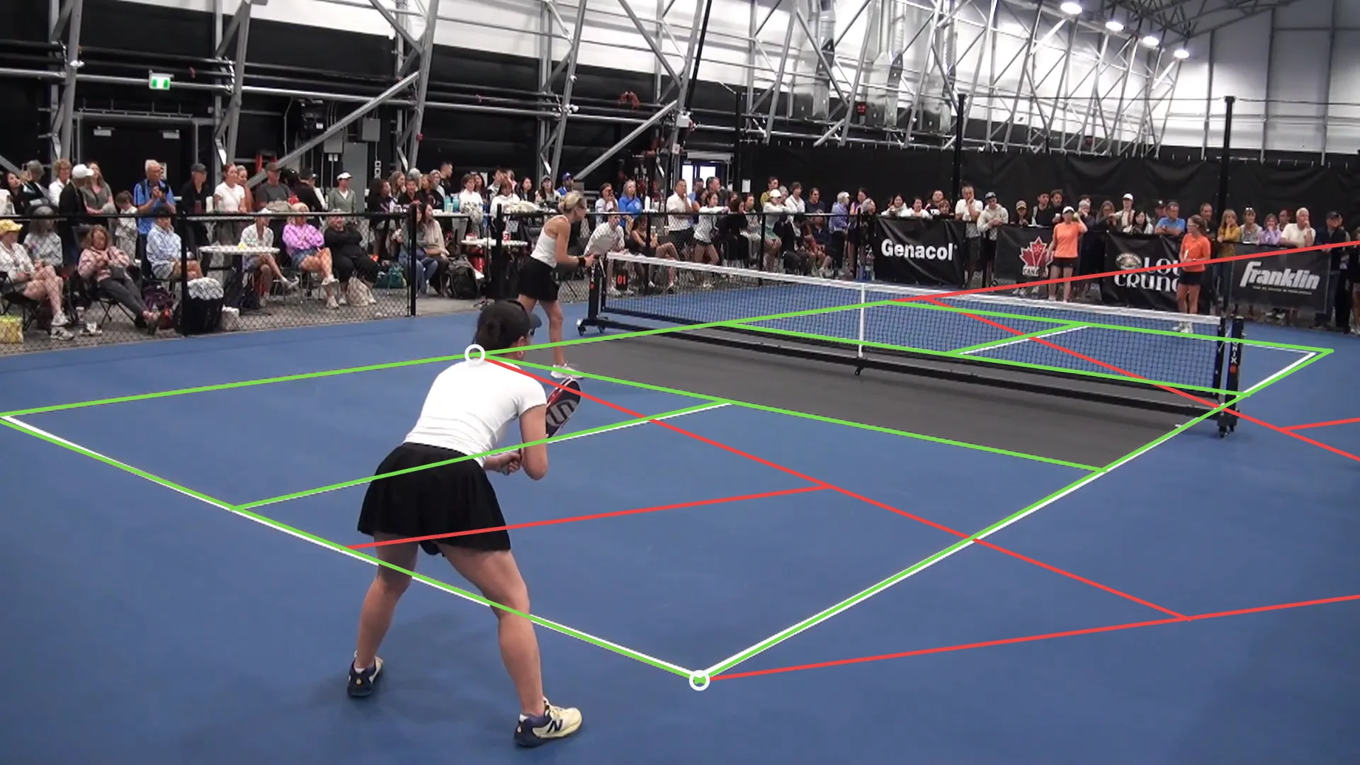
Lesson 2 of Image Alignment. Written on (x, y, 1), a 3×3 matrix can translate (affine, six numbers) and, once its last row is allowed to vary, make parallel lines meet (projective, eight numbers). On a pickleball court, an affine map fixed by three corners misses the fourth by 3.50 m; a homography through four lands the held-out centre-line corner 0.47 cm from the rulebook.
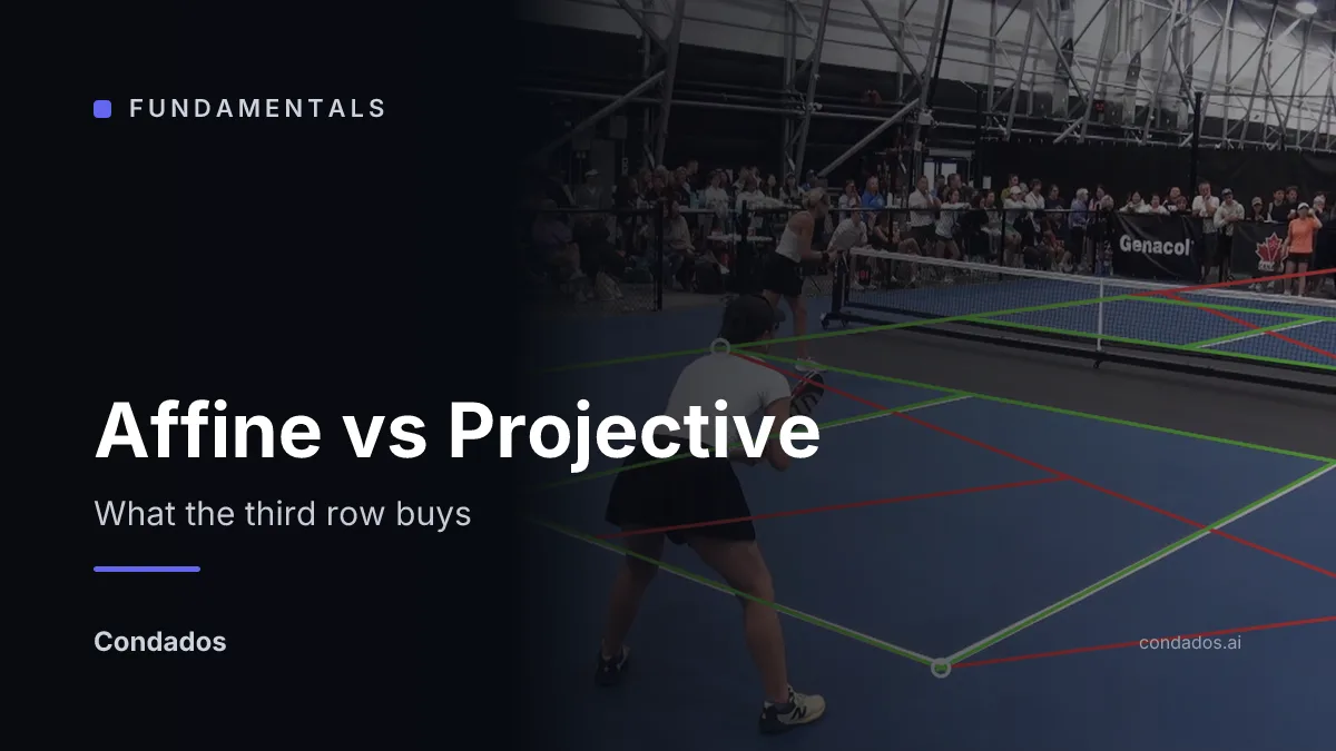
An affine transform can move, rotate, stretch and slant a picture, but lines that start parallel stay parallel. A perspective transform, or homography, can also make them converge, which is what a camera does to anything it sees at an angle.

Which one you need depends on the camera:

- Perspective: a document photographed at an angle, a projector aimed up at a wall (keystone correction), a court or a road seen from a camera beside it. Anything the camera sees obliquely.
- Affine is enough: a scanner or a microscope, where the view is straight on and only shift, rotation and scale change; satellite images taken looking straight down; two frames of video a moment apart, when the camera has barely moved.
Write each point as and a 3×3 matrix can do the two things a 2×2 could not. Its last column translates, which gives the six-number affine map. Letting its last row vary divides every output by a number that changes across the image, and that makes parallel lines meet: the eight-number projective map, or homography. On this court the difference is not subtle. An affine map fixed by three corners puts the fourth 3.50 m from where the paint is; a homography through four puts a corner it never saw 0.47 cm from the rulebook position.
Where we are
Part of image alignment. Lesson 1 showed that a 2×2 matrix cannot translate and cannot make parallel lines meet, and that on frame 45000 the best one misses every corner by 60 px. Both failures have the same fix, which is to use the extra coordinate from homogeneous coordinates.
First the last column: affine
Put the 2×2 in the top-left corner of a 3×3, a translation in the last column, and underneath:
The 1 at the end of the input picks up and , so translation is now part of the multiplication. Six numbers, so three point pairs fix it. It still keeps parallel lines parallel, since the bottom row leaves the last coordinate at 1 and the top two rows are the old 2×2 plus a shift [1].
Then the last row: projective
Now let the bottom row be anything, :
The output is divided by a number that depends on where you are. Far from the camera the divisor is large and things shrink; near it they grow. That is perspective, and it is also why parallel lines can meet: the divisor is zero along one line of the input, and that line goes to infinity in the output, or the other way round. Eight numbers (the ninth is the overall scale, which does not matter for the same reason and are the same point), so four point pairs fix it [2].
Hartley and Zisserman put these in a ladder: a similarity keeps shape and has four numbers, an affine map keeps parallelism and has six, a projective map keeps only straight lines and has eight [1].
Why a plane is exactly projective
This is not a lucky fit. The camera models post writes a pinhole camera as a 3×4 matrix acting on . Every point of the court has , so the third column never contributes, and what is left, , is a 3×3 acting on . The map from a plane to a pinhole image is a homography, with no approximation beyond the pinhole itself [3].
The same comparison on every piece of held-out evidence the unit uses, in centimetres:
| NBC | NKC | near centre line | far right sideline | far baseline | |
|---|---|---|---|---|---|
| affine, 3 corners | 91.6 | 188.5 | 125.6 | 397.0 | 308.8 |
| affine, least squares on 4 | 122.4 | 34.1 | 78.6 | 105.1 | 551.6 |
| homography, 4 corners | 0.47 | 5.63 | 2.66 | 5.95 | 38.4 |
Giving the affine map all four corners and a least-squares fit does not rescue it. It spreads its error over the four corners it was given (42 to 114 cm at each) and gets worse on the far baseline, 5.52 m, because the far court is where perspective matters most and an affine map has no way to express it.
import cv2
import numpy as np

court = np.float32([[0.0254, 0.0254], [0.0254, 6.0746], [4.6004, 0.0254], [4.6004, 6.0746]])
image = np.float32([[-18.52, 587.39], [987.25, 959.91], [669.68, 500.09], [1555.24, 663.22]])

A_img2court = cv2.getAffineTransform(image[:3], court[:3])      # 2x3, six numbers
H_img2court = cv2.getPerspectiveTransform(image, court)         # 3x3, eight numbers
nbc = np.float32([[[332.06, 717.24]]])
print(cv2.transform(nbc, A_img2court))                          # [[[0.0252 2.1339]]]
print(cv2.perspectiveTransform(nbc, H_img2court))               # [[[0.0254 3.0547]]]
#include <opencv2/imgproc.hpp>
#include <iostream>
int main() {
std::vector<cv::Point2f> court{{0.0254f, 0.0254f}, {0.0254f, 6.0746f}, {4.6004f, 0.0254f}, {4.6004f, 6.0746f}};
std::vector<cv::Point2f> image{{-18.52f, 587.39f}, {987.25f, 959.91f}, {669.68f, 500.09f}, {1555.24f, 663.22f}};
cv::Mat A = cv::getAffineTransform(image.data(), court.data()); // first three
cv::Mat H = cv::getPerspectiveTransform(image, court);
std::vector<cv::Point2f> nbc{{332.06f, 717.24f}}, a, h;
cv::transform(nbc, a, A);
cv::perspectiveTransform(nbc, h, H);
std::cout << a[0] << " " << h[0] << "\n";
}
Now you try
Start on Affine (3 pts). Drag the three white corners and watch the red model and the ghost of the fourth corner; the readout scores NBC and NKC in centimetres. Then switch to Homography (4 pts) and nudge one corner by a few pixels: the held-out error moves by centimetres near the camera, and the far-corner scale in the last line tells you why it moves by much more at the back.
Frame 45000 of "2026.07.25 WD Open … (Gold Medal match)" by pickleball4you, CC BY 3.0.
In the wild
A different court, outdoors, from a different camera, where both baseline corners are outside the frame and were found as line intersections [4]. The same two maps, the same held-out checks:
| outdoor court | NBC | NKC | near centre line |
|---|---|---|---|
| affine, 3 corners | 111.3 cm | 115.5 cm | 47.3 cm |
| homography, 4 corners | 0.77 cm | 11.3 cm | 2.66 cm |
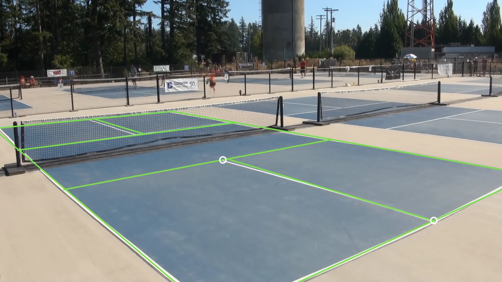
The homography beats the affine map by 145× at NBC, 10× at NKC and 18× along the centre line; indoors the same factors were 195×, 33× and 47×. The size of the gap depends on the camera and the geometry of the evidence. The ordering, affine metres against projective centimetres, does not change.
Where this breaks
A homography through four points reproduces those four points exactly, whatever they are. If one of the four was found 3 px off, the fit bends the whole court to pass through the wrong pixel without complaint, and the only sign is in the held-out numbers. Look at the far baseline in the table: 38.4 cm, the largest error the homography makes, coming from four corners that are each good to a fraction of a pixel.
Four points leave nothing over to average against, and nothing to detect a bad one with. What is needed is a way to use more than four, and to say how an error in each one turns into an error on the court.
Next
Lesson 3 writes the homography as eight linear equations in nine unknowns, solves them with the SVD for any number of point pairs, and follows the error from the pixel to the far baseline.
Run it: every code block on this page has a cell in the unit’s notebook, open it in Colab.
References
[1] Hartley, R., & Zisserman, A. (2004). Multiple View Geometry in Computer Vision (2nd ed.), §2.4 “A hierarchy of transformations”, p. 37. Cambridge University Press.
[2] Hartley, R., & Zisserman, A. (2004). Multiple View Geometry in Computer Vision (2nd ed.), §2.3 “Projective transformations”, p. 32. Cambridge University Press.
[3] Hartley, R., & Zisserman, A. (2004). Multiple View Geometry in Computer Vision (2nd ed.), ch. 13 “Scene planes and homographies”, p. 325. Cambridge University Press.
[4] pickleball4you (2024). 2024.08.30 MS4.0 Philip Wong vs Tristan Clark (Round Robin, match 6). YouTube, CC BY 3.0. youtube.com/watch?v=K0qrASvix3Y