
Before this unit: Homogeneous coordinates
Bird's-Eye View and Panoramas: Warping with a Homography
Lesson 5 of Image Alignment. Pushing each pixel forward through H leaves holes in 56% of the far court's bird's-eye view; pulling each output pixel back fills every one exactly once, and matches OpenCV's warpPerspective to one grey level. Interpolation decides what the pulled-back value is. Then a median of 31 warped frames removes the players, who cover 7% of the court in one frame.
With a homography in hand you can redraw a whole photograph as if it had been taken from somewhere else: straight down onto a court, flat onto a page, or joined onto the next photograph of a panorama.
The same two steps, move the pixels and then combine them, are behind:
- Bird’s-eye views of a court, a road or a car park, from a camera that sees them at an angle.
- Document scanning, where the page is warped to a rectangle.
- Panorama modes, where each photo is warped into a shared frame and the overlaps blended [3].
- Graphics on the ground in sport, where the graphic is warped onto the pitch and blended under the players:

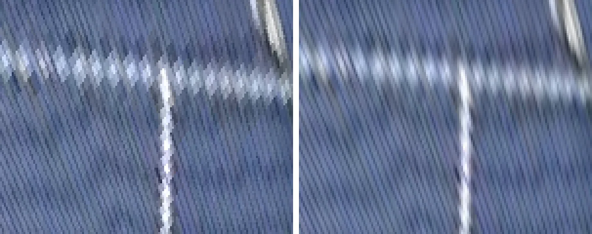
With a homography in hand, there are two ways to move an image through it, and only one works. Pushing every source pixel to where sends it leaves holes wherever the output is stretched: 56% of the far half of this court’s bird’s-eye view is never written. Pulling every output pixel back through writes each one exactly once. The value you pull lands between four source pixels, and interpolation decides how to mix them. Once several images share one output, blending decides how to combine them: a median of 31 frames removes the players, who cover 7.0% of the court in any single one.
Where we are
Part of image alignment. Lessons 2 and 3 produced a homography from the court’s plane to frame 45000, and RANSAC is how you get one when some of the point pairs are wrong. This lesson uses it: every pixel of a bird’s-eye view of the court, at 2 cm per pixel, is filled from the photograph.
Push or pull
The obvious way is forward: take each pixel of the frame, send it through , and write it where it lands. The trouble is that stretches the far court and squeezes the near one. Where it stretches, neighbouring source pixels land two or three output pixels apart and the gaps between them are never written. Where it squeezes, several land on the same output pixel and all but the last are thrown away.
Backward mapping turns the loop around. For each output pixel, apply to find
where it came from in the source, and read the source there. Every output pixel is
visited once and gets exactly one value. That is why warpPerspective and every
resampler like it work this way [1].
On the court, measured over the 205,569 top-view pixels the camera sees:
| forward mapping | near half | far half | whole court |
|---|---|---|---|
| pixels never written (holes) | 12.2% | 55.8% | 34.0% |
| pixels written more than once | 78.1% |
The near half is compressed, most of its output pixels hit several times, and still
leaves 12% unwritten; the far half is too sparse. The backward warp written out below and cv2.warpPerspective agree to a maximum
difference of 1 grey level, over every visible pixel.
What the pulled-back value is
A pulled-back position is almost never a whole pixel. Nearest neighbour takes the closest one. Bilinear takes the four around it and mixes them by how close each is, first along , then along [1].
import cv2
import numpy as np

frame = cv2.imread("frame_045000.png")
H_court2img = np.array([[214.196342, 90.15869, -26.259561],
                        [28.479672, -12.463675, 587.254072],
                        [0.095124, -0.077166, 1.0]])
s, m = 50, 1.5                                   # 50 px per metre, 1.5 m margin
H_court2top = np.array([[0, s, m * s], [-s, 0, (13.41 + m) * s], [0, 0, 1.0]])
H_img2top = H_court2top @ np.linalg.inv(H_court2img)

top = cv2.warpPerspective(frame, H_img2top, (455, 820), flags=cv2.INTER_LINEAR)
cv2.imwrite("topview.png", top)                  # backward mapping inside
#include <opencv2/imgcodecs.hpp>
#include <opencv2/imgproc.hpp>
int main() {
cv::Mat frame = cv::imread("frame_045000.png");
cv::Matx33d H_court2img(214.196342, 90.15869, -26.259561,
28.479672, -12.463675, 587.254072,
0.095124, -0.077166, 1.0);
const double s = 50, m = 1.5;
cv::Matx33d H_court2top(0, s, m * s, -s, 0, (13.41 + m) * s, 0, 0, 1);
cv::Matx33d H_img2top = H_court2top * H_court2img.inv();
cv::Mat top;
cv::warpPerspective(frame, top, H_img2top, {455, 820}, cv::INTER_LINEAR);
cv::imwrite("topview.png", top);
}
Blending: several images, one output
Stitching a panorama means several images land on the same output, and some rule has to combine them where they overlap. The simplest is to average, which ghosts anything that moved; feathering weights each image down towards its own edge; multiband blending does that separately for coarse and fine detail, so seams vanish without blurring [2], and it is what Brown and Lowe’s stitcher uses [3]. Szeliski covers the whole family under compositing [4].
A fixed camera gives the cleanest case to measure. The 31 frames either side of frame 45000 all share one homography, and a per-pixel median keeps whatever most of them agree on: the court, not the players. In frame 45000, 7.0% of the court’s bird’s-eye pixels differ from the median by more than 40 levels in some colour channel, and those pixels are the players and their shadows.
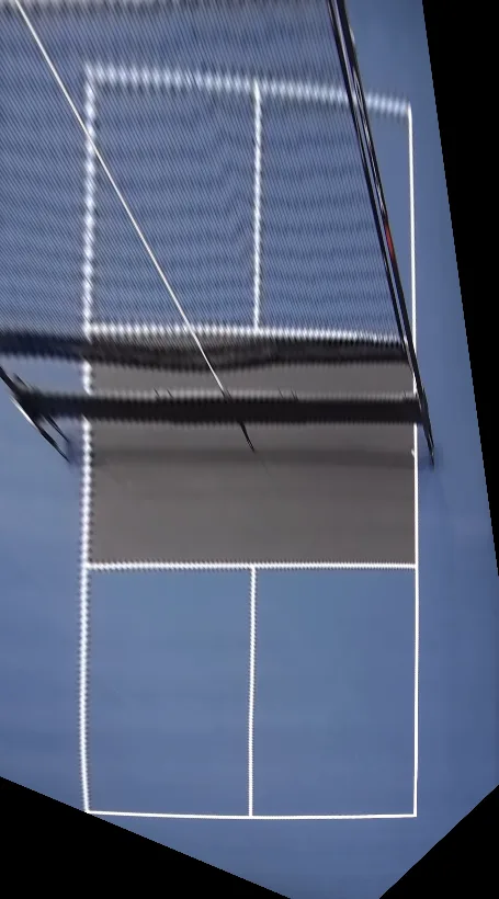
The order does not matter here, and in a panorama it does. Taking the median of the 31 frames first and warping once, or warping all 31 and taking the median, differs by a mean of 0.55 grey levels (99% of pixels within 2), which is interpolation rounding. It works because every frame has the same . In a panorama each image has its own, and the only place the images agree about where a pixel is is the output, so there you have to warp first and blend second.
Now you try
The Warp tab renders the bird’s-eye view live, pulling every output pixel back through the homography the four corners define. Drag a corner a few pixels and watch the far court swing while the near court barely moves: that is the scale map from lesson 3, seen as an image. Toggle Bilinear off to see nearest neighbour.
Frame 45000 of "2026.07.25 WD Open … (Gold Medal match)" by pickleball4you, CC BY 3.0.
In the wild

A panorama is where blending earns its place. Two photographs of Barcelona harbour taken from one spot on Montjuïc, panning right, published as source frames for a stitched panorama [5]. Everything in this unit, in order, at 1600 px wide: SIFT finds 6,788 and 8,197 keypoints, the ratio test keeps 1,011 matches, RANSAC keeps 906 of them (89.6%), and the DLT through those 906 reprojects them with a median error of 0.80 px. The second image is warped into the first’s frame by backward mapping.
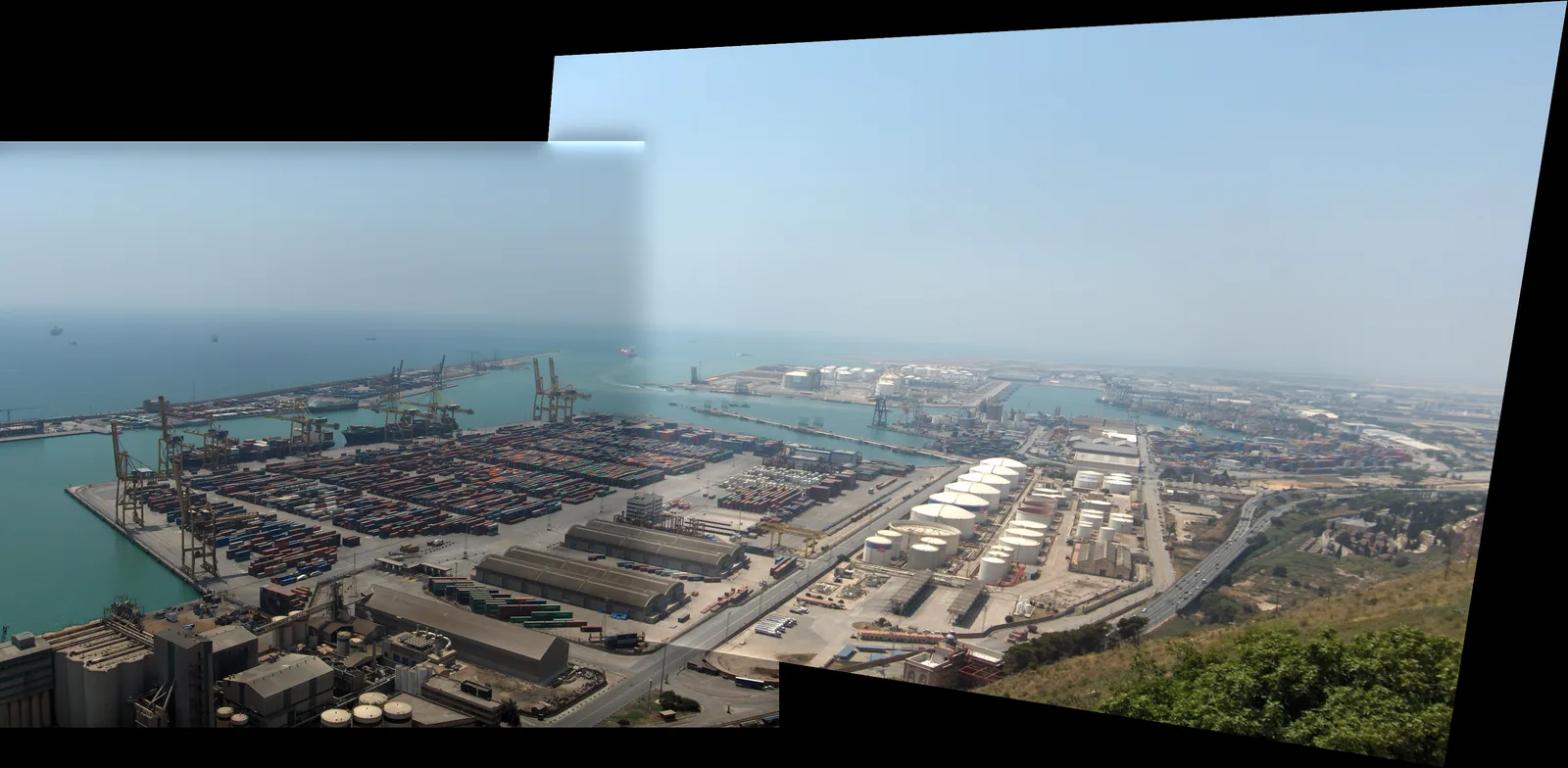
The second photograph is exposed brighter: over the overlap, the first’s mean brightness is 0.76 of the second’s. That is what a seam shows, and the three blends handle it very differently. Measured as the average brightness step across the seam line, against 4.9 grey levels for the same measure a few columns away where there is no seam:
| blend | step across the seam |
|---|---|
| hard cut | 40.5 grey levels |
| feather | 4.6 |
| multiband, 5 levels | 5.5 |
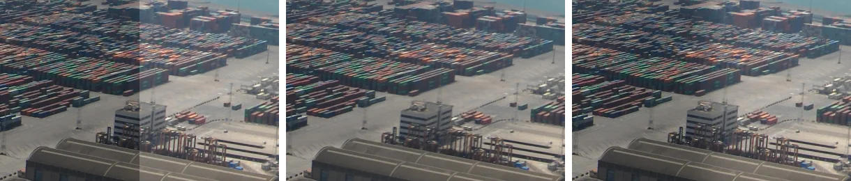
Feather and multiband both erase the step here, and feather scores slightly better on this one number. Where they differ is away from the seam line: feathering spreads the exposure difference across the whole overlap as a slow gradient, visible in the sky of the panorama above as a lighter band, while multiband blends the low frequencies over a wide zone and the fine detail over a narrow one [2]. The step metric only looks at the seam itself, which is one of this comparison’s limits.
Where this breaks
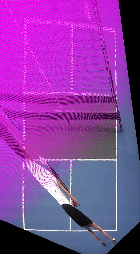
Only the plane is mapped correctly. A homography is exact for points on the court and wrong for everything else. The player in frame 45000 comes out of the warp smeared into a long streak away from the camera, because the warp treats her head as a point on the floor far behind her feet. The net is the same, which is why its mesh is printed across the far court above. In a panorama the same effect is called parallax: step sideways between shots and anything off the dominant plane ghosts, whatever the blending.
The lens is not a pinhole, and the warp carries its bend into the output. The unit hub measures how much: the near baseline bows by 7.7 px, and a one-parameter correction cuts the far-sideline error from 5.95 cm to 1.96.
Next
That is the end of the unit: a map from a plane in one image to a plane anywhere else, computed from point pairs, made robust, and used. When the scene is not a plane, one 3×3 no longer describes it, and the tools are the ones in structure from motion. The unit’s hub collects every number and its limits in one place.
Run it: every code block on this page has a cell in the unit’s notebook, open it in Colab.
References
[1] OpenCV (5.x, commit a0cda08). warpPerspective, documentation comment in modules/imgproc/include/opencv2/imgproc.hpp, which defines each output pixel as the source sampled at M applied to (x, y), with M inverted first unless WARP_INVERSE_MAP is set. github.com/opencv/opencv
[2] Burt, P. J., & Adelson, E. H. (1983). A Multiresolution Spline with Application to Image Mosaics. ACM Transactions on Graphics, 2(4), 217–236. doi:10.1145/245.247
[3] Brown, M., & Lowe, D. G. (2007). Automatic Panoramic Image Stitching using Invariant Features. International Journal of Computer Vision, 74(1), 59–73. doi:10.1007/s11263-006-0002-3
[4] Szeliski, R. (2022). Computer Vision: Algorithms and Applications (2nd ed.), §8.4 “Compositing”, including §8.4.2 “Pixel selection and weighting (deghosting)” and §8.4.4 “Blending”. Springer. Free PDF
[5] Pap3rinik (2006). BarcelonaHarbour1.jpg and BarcelonaHarbour2.jpg. Wikimedia Commons, public domain. commons.wikimedia.org
