
geometry
18 posts · browse all tags
 Fundamentals
Lowe's Ratio Test: Matching Features You Can Trust
How SIFT matches points between two photos: pair each descriptor with its nearest neighbour, then keep the pair only when the second-nearest is clearly farther. On the Barcelona harbour pair, scored against a homography fitted by a different detector, the ratio test at 0.75 keeps 440 matches of which 420 are right; an absolute distance threshold tuned to keep the same 440 gets 391 right. Built in NumPy and checked against OpenCV's BFMatcher.
 Fundamentals
Scale Space and the Difference of Gaussians
Scale space is a stack of copies of a photo, each blurred a little more, which lets a detector find features of every size and say how big each one is. Discs of radius 4, 8 and 16 px answer most strongly at a blur of 2.77, 5.61 and 11.34 px, close to r/√2; subtracting neighbouring blurs reproduces the scale-normalized Laplacian with a correlation of 0.99; and on a harbour photo SIFT's 9 octaves give each point a size that halves when the photo does.
 Fundamentals
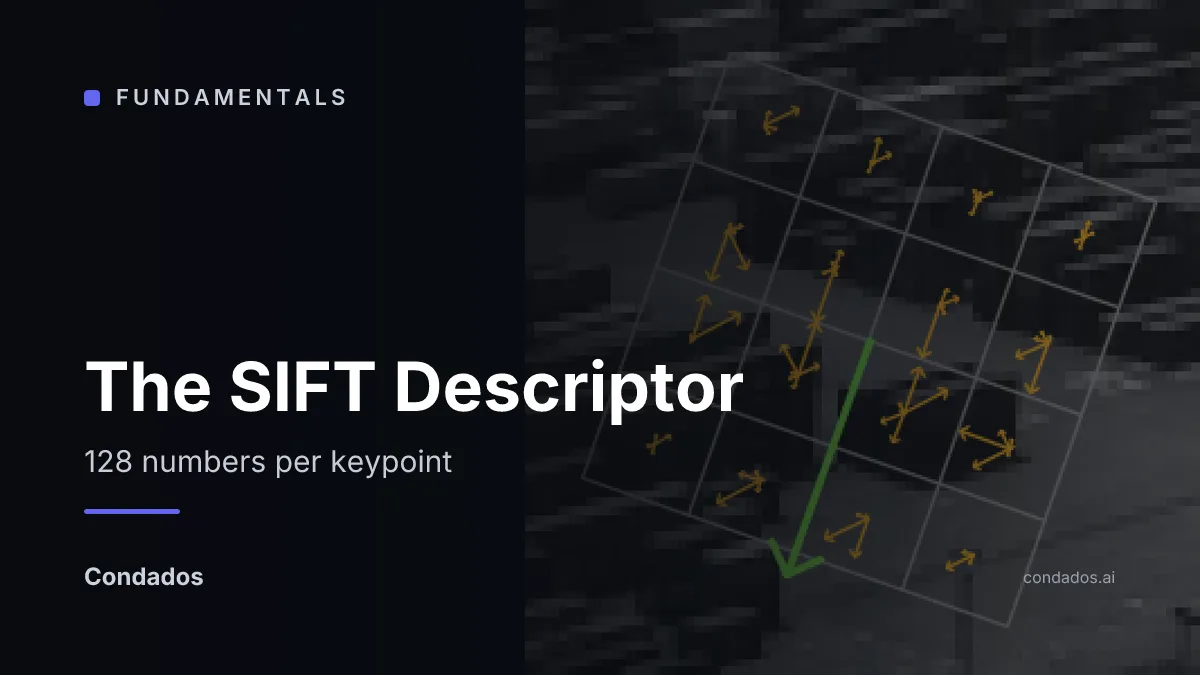
The SIFT Descriptor: 128 Numbers per Keypoint
How SIFT describes the neighbourhood of a keypoint with 128 numbers that come out the same in another photo: gradient histograms on a 4×4 grid, turned to the keypoint's own direction, normalized and clipped. Each step tested by removing it on a photo of Barcelona harbour: without the direction, matches against a copy turned 45° fall from 1,927 correct to 0; without normalization, a contrast change takes them from 907 to 146.
 Fundamentals
How SIFT Finds Keypoints: Extrema, Refinement, Orientation
How SIFT turns a stack of blurred photos into a short list of points it can find again: every point that beats its 26 neighbours, a sub-pixel fit, a contrast test, an edge test and a direction for each survivor. Built from scratch on a photo of Barcelona harbour, where 7,053 candidates become 2,896 points and 3,510 keypoints, and checked against OpenCV keypoint for keypoint.
 Fundamentals
What Makes a Good Keypoint? Repeatability, Measured
A good keypoint is one a detector finds again in another photo of the same scene, in the same place and at the same size. Measured on a harbour photo under known turns, zooms, blur and noise: on position alone Harris corners and SIFT points come back about equally often, and which one leads depends on the tolerance; what SIFT adds is a size that follows the zoom, which takes correct matches across a 2× zoom from 1 to 294.
 Fundamentals
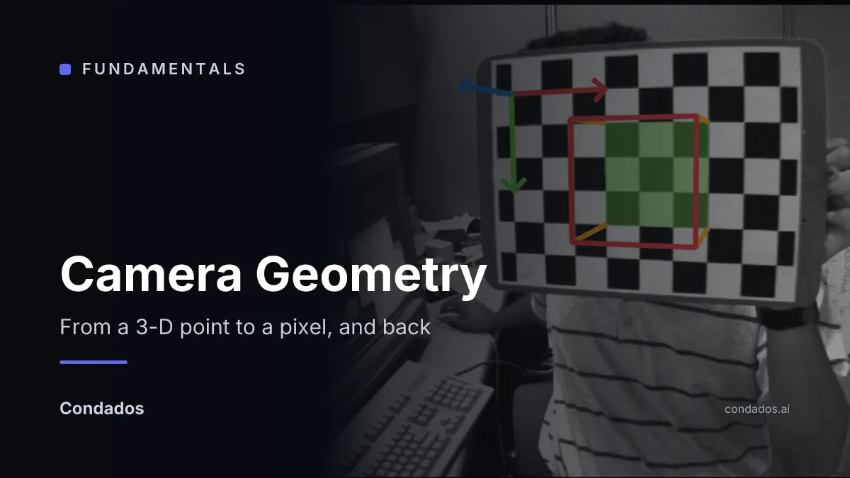
Camera Geometry: From a 3-D Point to a Pixel, and Back to the Camera
How a camera sends any point of the world to a pixel with one matrix, and how running that matrix backwards gives you the camera's focal length and where it stood. One pipeline, from a point on a chessboard to a pixel to a calibration and a pose, measured on OpenCV's own thirteen photographs of a board.
 Fundamentals
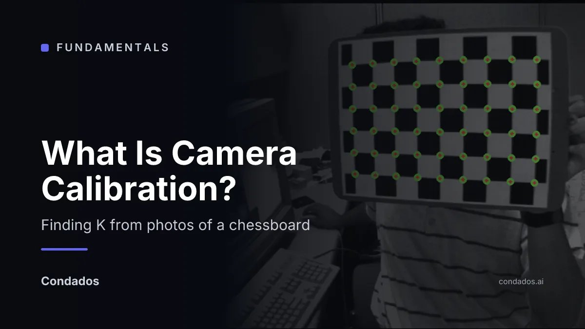
What Is Camera Calibration? Finding K from Photos of a Chessboard
Lesson 3 of Camera Geometry. Calibration measures a camera's focal length, image centre and lens bend by fitting the camera model to photos of a flat board whose corners are known. On OpenCV's thirteen chessboard photos: 0.41 px of reprojection error, a held-out photo that scores like the fitted ones, and a focal length anywhere from 520 to 568 px if only three photos are used.
 Fundamentals
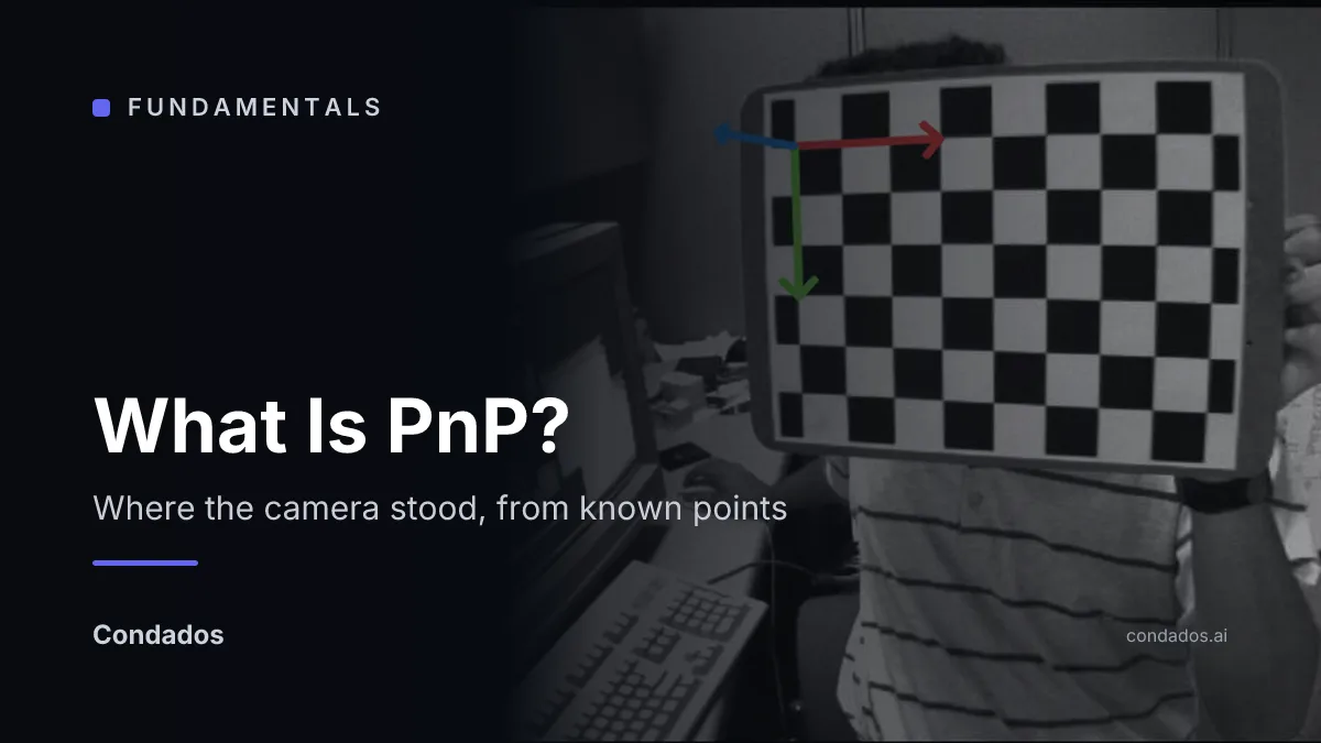
What Is PnP? Finding Where the Camera Is from Known Points
Lesson 4 of Camera Geometry. PnP finds where a calibrated camera stood and which way it faced from points whose positions are known and where they appear in one photo. On OpenCV's chessboard photos it returns the calibration's own pose to 0.00002°, four corners are enough for 0.27 px, and with five corners found wrong a plain fit moves the camera 2.5 squares where RANSAC moves it 0.008.
 Fundamentals
Rotate, Scale, Shear: Images as 2×2 Matrices
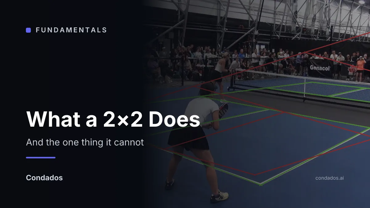
Lesson 1 of Image Alignment. A 2×2 matrix is where it sends the two axes; its determinant is how much it scales area and its SVD is rotate, stretch, rotate. The one thing it cannot do is make parallel lines meet. On a pickleball court, the sidelines are 20.35° apart in the photograph, so the best 2×2 misses every corner by 60 px.
 Fundamentals
Affine vs Perspective Transform
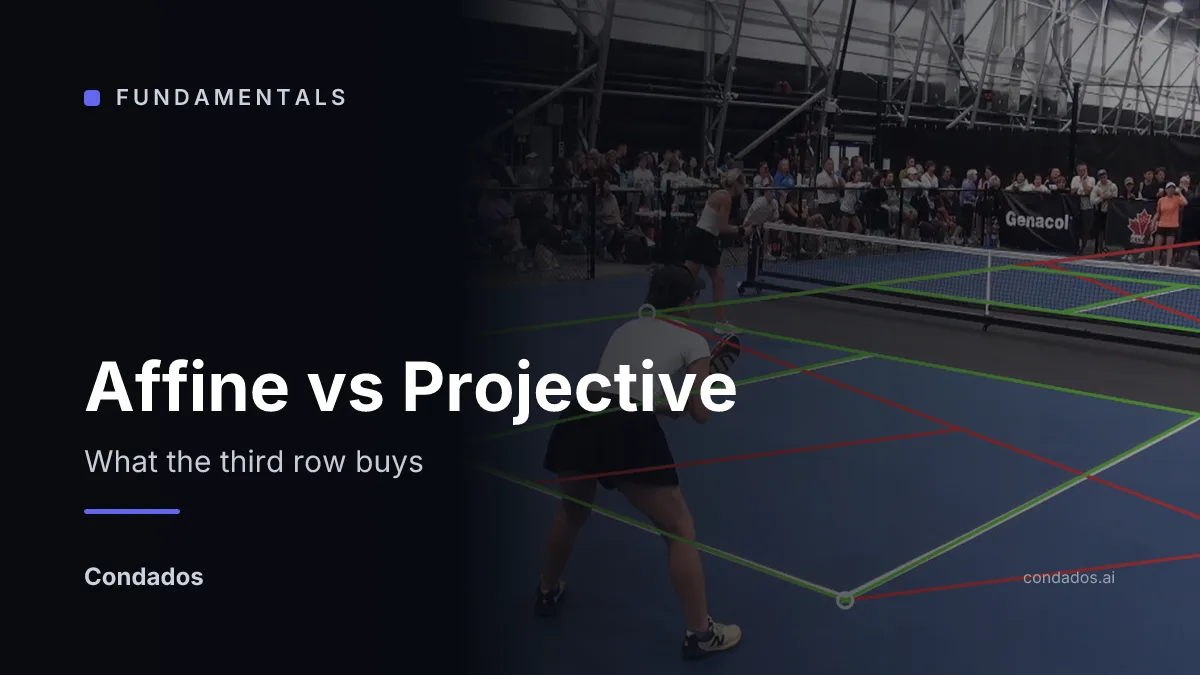
Lesson 2 of Image Alignment. Written on (x, y, 1), a 3×3 matrix can translate (affine, six numbers) and, once its last row is allowed to vary, make parallel lines meet (projective, eight numbers). On a pickleball court, an affine map fixed by three corners misses the fourth by 3.50 m; a homography through four lands the held-out centre-line corner 0.47 cm from the rulebook.
 Fundamentals
How to Compute a Homography from Four Points
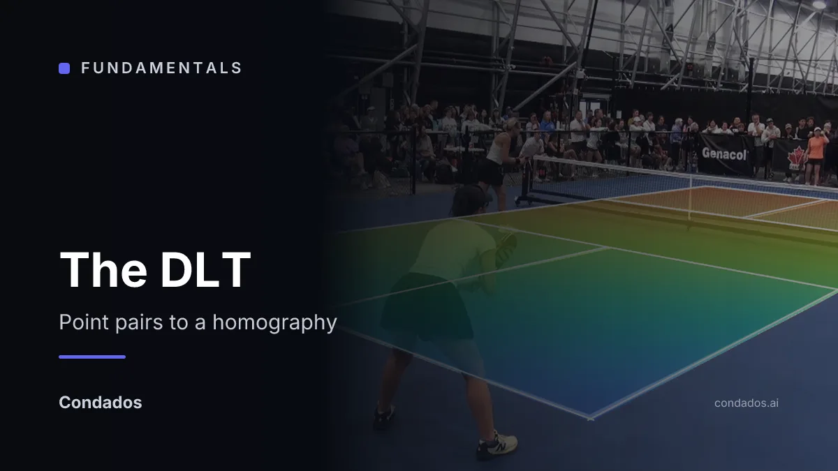
Lesson 3 of Image Alignment. Each point pair gives two linear equations in the nine entries of H, and the answer is the singular vector of the smallest singular value. Normalising the coordinates drops the condition number from 53,466 to 6.4, and on this court changes the answer by under 0.2 cm. What decides the error is where the pixels are: one pixel is 0.6 cm of court at the near baseline and 8.1 cm at the far one.
 Fundamentals
Homogeneous Coordinates: Why Vision Adds a 1
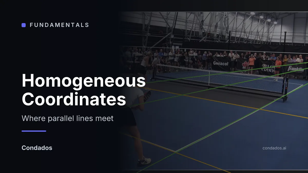
Lesson 1 of Camera Geometry, and the prerequisite of Image Alignment. Add a third coordinate and a point becomes a ray, a line becomes a 3-vector, and both the line through two points and the point where two lines cross are one cross product. Measured on a pickleball court: a corner 18.5 px outside the frame, found anyway, and two sidelines that are parallel on the ground meeting 2,252 px to the right.
 Fundamentals
Bird's-Eye View and Panoramas: Warping with a Homography
Lesson 5 of Image Alignment. Pushing each pixel forward through H leaves holes in 56% of the far court's bird's-eye view; pulling each output pixel back fills every one exactly once, and matches OpenCV's warpPerspective to one grey level. Interpolation decides what the pulled-back value is. Then a median of 31 warped frames removes the players, who cover 7% of the court in one frame.
 Fundamentals
What Is a Homography?
How to take a photo of anything flat, a court, a page, a wall, and work out where on it every pixel lies. One pipeline, from painted lines to corners to a 3×3 map to a bird's-eye view, and why a simpler map cannot do it: measured on one frame of a pickleball final, an affine map misses the far sideline by 3.97 m where a homography misses it by 6 cm.
 Fundamentals
RANSAC: How Vision Algorithms Vote Away Outliers
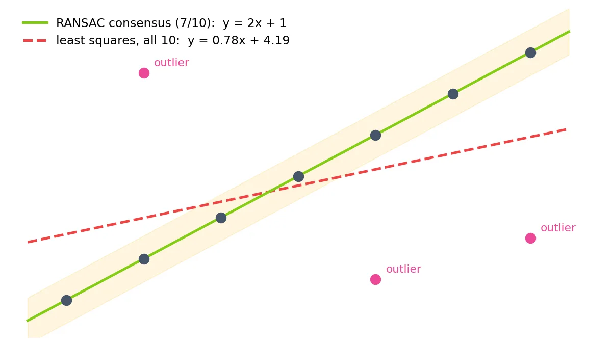
RANSAC separates data into inliers and outliers by fitting models to random minimal samples and keeping the one with the largest consensus. Walked end to end on two vision problems: a walking-speed estimate that three false detections drag from 2.00 m/s to 0.78, and a basketball shot called from a 3-point parabola fit. Plus the one-line formula for how many samples you need, a hands-on lab, and real inlier ratios measured on the temple dataset.
 Fundamentals
What Is SIFT? Finding the Same Point in Two Photos
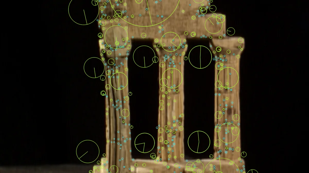
SIFT finds points in one photo that can be found again in another photo of the same scene, and describes each with 128 numbers so the two can be paired. One pipeline, from blurring at many sizes to keeping only the unambiguous pairs, run on two photos of Barcelona harbour and scored against a homography fitted by a different detector: 420 of the 440 pairs it keeps are right, and the five lessons take each step apart.
 Fundamentals
Structure from Motion, from Scratch: 47 Photos to a 3-D Temple in ~800 Lines of Python
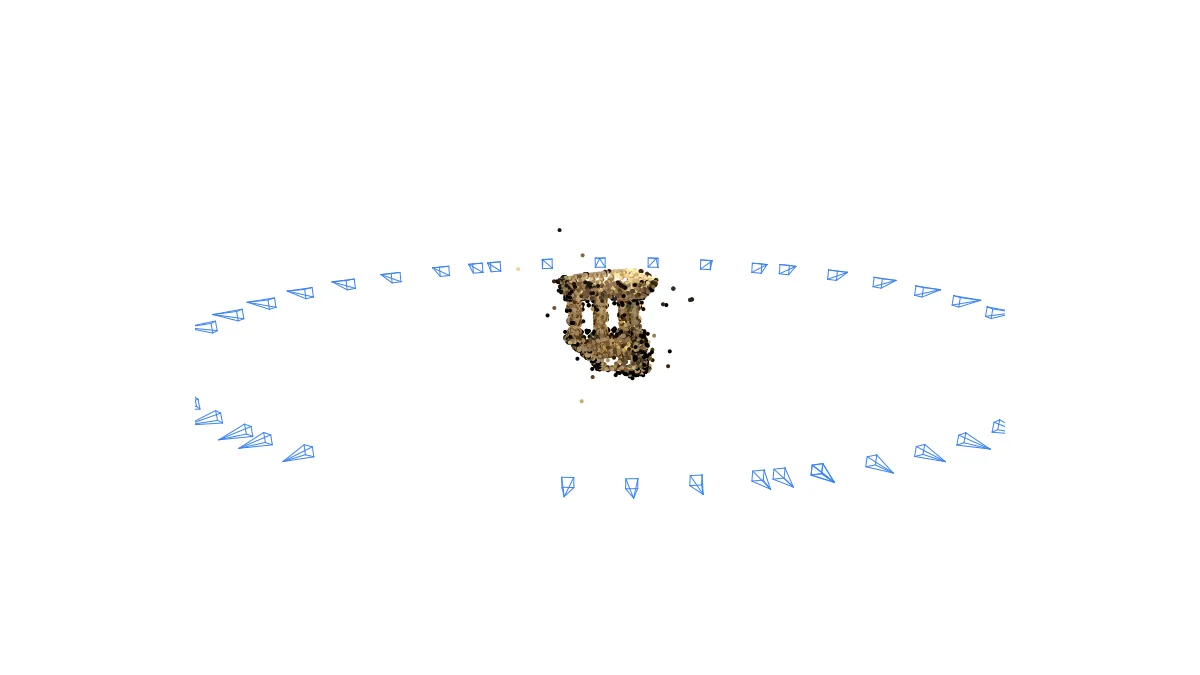
How overlapping 2-D photos become 3-D points and camera poses: SIFT matching, the essential matrix, triangulation, PnP growth, and sparse bundle adjustment, built from scratch with OpenCV + SciPy. The pipeline registers all 47 Middlebury temple views at 0.25 px mean reprojection error, next to COLMAP's 0.30 px on the same images. Worked examples, three interactive labs, and the reconstruction growing image by image.
 Fundamentals
The Camera Matrix: K, [R|t] and P, Worked on a Real Chessboard
Lesson 2 of Camera Geometry. A camera is one 3×4 matrix: the focal lengths and image centre in K, where the camera stands in [R|t], and their product P, which sends any point of the world to a pixel. Worked on one corner of a chessboard in OpenCV's own calibration photos, checked against cv2.projectPoints, and taken apart again.