
Before this unit: Edge detection
Lowe's Ratio Test: Matching Features You Can Trust
How SIFT matches points between two photos: pair each descriptor with its nearest neighbour, then keep the pair only when the second-nearest is clearly farther. On the Barcelona harbour pair, scored against a homography fitted by a different detector, the ratio test at 0.75 keeps 440 matches of which 420 are right; an absolute distance threshold tuned to keep the same 440 gets 391 right. Built in NumPy and checked against OpenCV's BFMatcher.

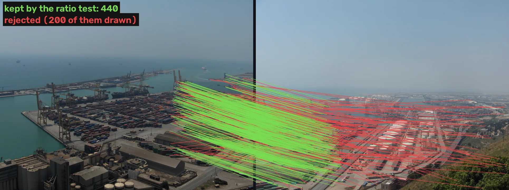
Matching finds, for each point in one photo, the point in another photo that shows the same thing, and the ratio test throws away the pairs that could equally have gone to a different point. The animation runs it on two photos of Barcelona harbour: every SIFT point is paired with its closest descriptor in the other photo, then the ratio test keeps the pairs it trusts.
- Describe. Every point in both photos already carries 128 numbers from lesson 4.
- Find the two nearest. For each point of photo A, the point of photo B whose 128 numbers are closest (distance ), and the runner-up ().
- Divide. The ratio says how much better the best candidate is than the next one.
- Keep the clear winners. A pair survives when the ratio is below a threshold, 0.75 here.
- Hand over to geometry. What survives still knows nothing about how the camera moved; RANSAC checks that next.
You have met it in:
- Panorama apps, which match points between neighbouring photos before stitching them (unit 3.5 stitches this same pair).
- 3-D reconstruction from photos, where every pair of photos is matched this way before structure from motion places the cameras.
- Visual place recognition and landmark search, which compare a photo’s features against a database and keep only unambiguous hits.
- AR and robot navigation, which match features from one frame to the next.
Comparing the best match with the second best is what makes a match trustworthy. On the Barcelona pair, the ratio test at 0.75 keeps 440 pairs and 420 of them are right. A threshold on the distance itself, tuned after the fact to keep the same 440, gets 391 right.
Where we are
Lesson 5, the last, of SIFT: step 6 of the unit’s pipeline. Lesson 1 set the yardstick, lessons 2 and 3 found the points with a size and a direction, and lesson 4 turned each one into 128 numbers. This lesson pairs those numbers across two photos.
Nearest neighbour
Two descriptors that describe the same patch of harbour should be close: the 128 numbers barely change when the camera turns a little or the light shifts, which is what lesson 4 built them for. “Close” is the straight-line (Euclidean) distance between the two lists of 128 numbers, treated as points in a 128-dimensional space. For each point of photo A, the candidate partner is the point of photo B at the smallest distance.
Every point gets a nearest neighbour, including the points of photo A that photo B does not show at all. Of photo A’s 2,897 points, only 755 land inside photo B (the two photos overlap on part of the harbour), so at least 2,142 nearest neighbours are wrong before anything is measured. Over all 2,897, nearest neighbour alone is right for 442: 15%.
Scoring a match without trusting SIFT
A match is right when photo B’s point sits where the harbour point of photo A appears in photo B. Both photos were taken from one spot on Montjuïc, turning the camera, so a single homography (the 3×3 map of unit 3.5) sends every pixel of A to its place in B. I fit that homography with ORB, a different detector with a binary descriptor [5], and a robust fit that ignores bad pairs: 453 ORB matches, 345 of them consistent, with a median error of 0.81 px. A SIFT match counts as right when its point in B lies within 3 px of where the ORB homography puts it. SIFT is never scored against itself, and the homography SIFT’s own matches give agrees with ORB’s to a median of 0.46 px (1.53 px at worst) over the 418 points it keeps.
One threshold on the distance does not work
The obvious rule keeps a pair when its distance is small. The trouble is that “small” depends on the patch. A textured patch with a unique look can sit far from its partner (lighting, a little perspective) and still be right, while a patch of repeated texture, such as a row of identical containers, has a partner at a small distance and three more as close.
Measured at equal count: the 440 pairs with the smallest distances (everything below 162.7) hold 391 right ones. The ratio test, keeping the same number, holds 420. Mikolajczyk and Schmid found the same ordering across many descriptors and photo pairs: the distance ratio gave higher precision than a threshold on the distance, and SIFT gained the most from it [3].
The ratio test
Lowe’s fix compares each candidate with the runner-up [1]. If the nearest descriptor is much closer than the second, the match is distinctive; if the two are close to each other, the point has lookalikes and either answer could be wrong. The rule keeps a pair when
with between 0.6 and 0.8 in practice. Lowe chose 0.8 on his data, where it removed 90% of the false matches while discarding less than 5% of the correct ones (§7.1 “Keypoint matching” [1]). This track uses 0.75, as unit 3.5 and the structure from motion post do.
The histogram below shows why the test works. Each match in the overlap is one count, at its ratio, coloured by the ORB check. The right ones have a median ratio of 0.28 and 82% of them sit below 0.5; the wrong ones have a median of 0.96 and 81% sit above 0.9, because a wrong partner is usually one of several equally poor candidates.
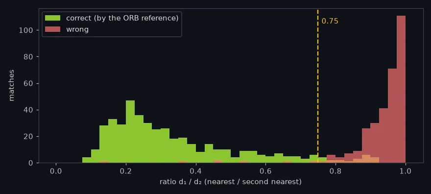
The threshold trades how many matches survive against how many of them are right:
| ratio threshold | 0.6 | 0.7 | 0.75 | 0.8 | 0.9 | none |
|---|---|---|---|---|---|---|
| kept | 395 | 422 | 440 | 490 | 809 | 2,897 |
| right | 389 | 411 | 420 | 426 | 438 | 442 |
| precision (right / kept) | 98.5% | 97.4% | 95.5% | 86.9% | 54.1% | 15.3% |
| share of the 442 right ones kept | 88% | 93% | 95% | 96% | 99% | 100% |
From 0.75 to 0.8 the test keeps 50 more pairs and only 6 of them are right. From 0.75 down to 0.6 it loses 45 pairs and 31 of those were right.
Now you try
The lab holds every point of photo A that photo B can show, with its two distances. Slide the threshold and watch the counts; tap a point on photo A to see its two candidates and its ratio. Find the threshold where the first wrong match appears, then the one where right matches start to disappear faster than wrong ones.
Cross-checking, the other common filter
The usual alternative asks whether the match is mutual: A’s point picks B’s point as its nearest,
and B’s point picks A’s back. On this pair, cross-checking alone keeps 1,050 pairs with
435 right (41%): it removes the points that many points of A pile onto, and keeps a mutual
pair even when it is one of two lookalikes. Both filters together keep 437 with 419 right, almost
the ratio test alone. OpenCV’s BFMatcher offers cross-checking as crossCheck=True [4]; the ratio
test needs knnMatch(k=2) and one line of Python.
How close is this to OpenCV?
The check: find the two nearest neighbours of every descriptor with NumPy, and compare the
distances with cv2.BFMatcher.knnMatch. The cells fetch the WebP copies of the two photos the page serves,
while the tables above come from the experiment scripts run on the original JPEGs, so the counts
differ.
import numpy as np
import cv2

a = cv2.imread("barcelona-a.webp", cv2.IMREAD_GRAYSCALE)
b = cv2.imread("barcelona-b.webp", cv2.IMREAD_GRAYSCALE)
sift = cv2.SIFT_create()
ka, da = sift.detectAndCompute(a, None)
kb, db = sift.detectAndCompute(b, None)
print("points:", len(ka), len(kb))

# squared distances, all pairs: |a|^2 + |b|^2 - 2 a.b
d2 = ((da**2).sum(1)[:, None] + (db**2).sum(1)[None]
      - 2 * da @ db.T)
d = np.sqrt(np.maximum(d2, 0))
order = np.argsort(d, axis=1)[:, :2]
rows = np.arange(len(da))
d1_np = d[rows, order[:, 0]]
d2_np = d[rows, order[:, 1]]

knn = cv2.BFMatcher(cv2.NORM_L2).knnMatch(da, db, k=2)
d1_cv = np.array([m.distance for m, n in knn])
d2_cv = np.array([n.distance for m, n in knn])
same = np.mean(order[:, 0] == [m.trainIdx for m, n in knn])
print("same nearest point:", round(100 * same, 2), "%")
print("largest d1 difference:",
round(float(np.abs(d1_np - d1_cv).max()), 4))points: 3492 3638 same nearest point: 100.0 % largest d1 difference: 0.0
The second cell scores the pairs with the same answer key as the tables: the homography ORB
gave, written by the experiment scripts as reference-homography.json.
import json

H = np.array(json.load(
    open("reference-homography.json"))["H_a_to_b"])
pa = np.float32([k.pt for k in ka])
pb = np.float32([kb[i].pt for i in order[:, 0]])
proj = cv2.perspectiveTransform(pa[None], H)[0]
right = np.linalg.norm(proj - pb, axis=1) <= 3
ratio = d1_np / d2_np
for t in (0.6, 0.75, 0.8, 1.01):
    keep = ratio < t
print(f"t={t}: kept {keep.sum()}, right {(keep & right).sum()}")t=0.6: kept 395, right 381 t=0.75: kept 468, right 430 t=0.8: kept 518, right 441 t=1.01: kept 3492, right 465
These cells keep OpenCV’s raw output, where a point with two strong directions appears twice (lesson 3), so they count about 3,500 points where the tables count 2,897 distinct ones.
In the wild
Barcelona’s two photos share a viewpoint, so only the camera’s direction changes between them. Walking around an object changes what the camera sees, and the ratio test then has less to keep. On Middlebury’s templeRing [7], 47 photos of a plaster temple taken every 7.66° around it, photo 1 matched against the next twelve:
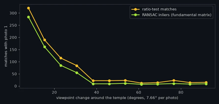
| viewpoint change | 7.7° | 15.3° | 23.0° | 30.6° | 38.3° | 46.0° | 91.9° |
|---|---|---|---|---|---|---|---|
| ratio-test matches | 321 | 190 | 115 | 84 | 22 | 22 | 15 |
| RANSAC inliers | 284 | 161 | 85 | 55 | 9 | 9 | 9 |
What it means: on the temple the ratio test keeps a usable set up to about 30° (55 pairs that agree on one geometry), and by 38° it keeps a handful that barely agree. Lowe’s own advice is to capture views of an object at least every 30° (§2 “Related research” [1]). On Barcelona, where the viewpoint did not move, 95.5% of what the ratio test keeps is right.
Where this breaks
Repeated structure. A harbour of identical containers, a building of identical windows: the true partner has twins at the same distance, the ratio goes to 1 and the pair is thrown away even when the nearest one is right. The ratio test loses those points instead of getting them wrong.
It is not one-to-one. Several points of A can keep the same point of B. Cross-checking or RANSAC removes those later.
It knows nothing about geometry. At 0.75, 20 of the 440 kept pairs are wrong. The homography fitted on SIFT’s own pairs throws out 22 as inconsistent. Removing those is the job of RANSAC, the next step.
Brute force grows with both photos. 2,897 × 3,109 distances of 128 numbers each, 9 million, is fine for two photos and too slow for a database of millions; approximate nearest-neighbour search trades a little accuracy for speed there (Szeliski §7.1.3 [2]).
One photo pair. The 0.75 trade-off above is for one pair from one viewpoint. Lowe’s 0.8 came from a different data set; the threshold is worth re-checking on your own photos.
What this means for your pipeline
- Use the ratio, not a distance cut. At equal count it kept 420 right pairs against 391.
- Start at 0.75. On this pair it keeps 95% of the right matches at 95.5% precision; 0.8 adds 50 pairs of which 6 are right, and 0.6 loses 31 right pairs.
- Follow it with RANSAC. 20 of the 440 kept pairs are still wrong.
- Expect fewer matches as the viewpoint moves. On the temple, consistent pairs fall from 55 at 30.6° to 9 at 38.3°; take photos closer together than that.
Exercises
- Write the test.
keep(d1, d2, t)returnsTruewhen the pair survives. Use the worked example’s two pairs to test it.
def keep(d1, d2, t):
    return True  # compare d1 / d2 with t

print(keep(24.4, 284.1, 0.75), keep(252.3, 252.4, 0.75))- Predict, then run. In the scoring cell, change the thresholds to 0.75 and 0.8. Before running: of the extra pairs 0.8 keeps, more than half right, or fewer?
- Break it. Replace the ratio test with an absolute threshold,
keep = d1_np < c, and choosecso it keeps the same number of pairs as 0.75. How many are right?
What you should see
These come from section 6 of the unit notebook, sift.ipynb, and from the cells on this page,
which count OpenCV’s raw points on the served WebP copies (so the numbers differ from the
tables above).
True Falseonce the comparison isd1 / d2 < t. The third check, 60/80 = 0.75, is not kept, because it is not below the threshold.- Fewer: 0.75 keeps 468 pairs with 430 right, 0.8 keeps 518 with 441. Of the 50 extra pairs, 11 are right.
- A threshold of about 167 keeps the same 468 pairs, and 384 of them are right, against 430 for the ratio test.
Check yourself
Four questions on this lesson. Pick an answer to see why it is right or wrong.
A point of photo A has its nearest descriptor in photo B at distance 252.3 and the second nearest at 252.4. What does the ratio test do?
The test compares the best candidate with the runner-up, not with a fixed distance. Two candidates at the same distance mean lookalikes, and on this pair the nearest one was wrong.
Kept at equal count (440 pairs), how many are right with the ratio test and with a threshold on the distance itself?
A textured point can sit far from its right partner and a repeated one close to a wrong one, so a single distance cut mixes them up; the ratio adapts to each point.
Moving the threshold from 0.75 to 0.8 on the Barcelona pair keeps 50 more pairs. How many of them are right?
Right matches pile up at low ratios and wrong ones near 1, so the pairs added between 0.75 and 0.8 are mostly wrong: 420 right of 440 becomes 426 of 490.
After the ratio test at 0.75, 20 of the 440 kept pairs are still wrong. What removes them?
The ratio test knows nothing about geometry. A homography fitted with RANSAC on SIFT’s own pairs throws out 22 as inconsistent.
Next
This closes the unit. SIFT puts the five lessons side by side with what the unit measured and its limits. The matches go on to RANSAC, which keeps the ones that agree on one geometry, and to the panorama of unit 3.5, built from this same pair.
Run it: every code block on this page has a cell in the unit’s notebook, open it in Colab.
Further reading
- Lowe 2004, §7.1 “Keypoint matching” [1], for the experiment behind the 0.8 threshold and the probability curves of right and wrong matches it was read from.
- Szeliski §7.1.3 “Feature matching” [2], for matching strategies beyond brute force and how to evaluate them.
- Mikolajczyk and Schmid [3], for a comparison of descriptors under the same kind of test, on many more photo pairs.
- RANSAC, for the geometric check that finishes what the ratio test starts.
References
[1] Lowe, D. G. (2004). Distinctive Image Features from Scale-Invariant Keypoints. International Journal of Computer Vision, 60(2), 91–110; §2 “Related research” and §7.1 “Keypoint matching”. doi:10.1023/B:VISI.0000029664.99615.94
[2] Szeliski, R. (2022). Computer Vision: Algorithms and Applications (2nd ed.), §7.1.3 “Feature matching”, p. 441. Springer. Free PDF
[3] Mikolajczyk, K., & Schmid, C. (2005). A Performance Evaluation of Local Descriptors. IEEE Transactions on Pattern Analysis and Machine Intelligence, 27(10), 1615–1630. doi:10.1109/TPAMI.2005.188
[4] OpenCV 4.11.0 source, modules/features2d/include/opencv2/features2d.hpp: BFMatcher(int normType=NORM_L2, bool crossCheck=false) and the crossCheck documentation (lines 1253–1268), commit 31b0eee.
[5] Rublee, E., Rabaud, V., Konolige, K., & Bradski, G. (2011). ORB: An Efficient Alternative to SIFT or SURF. ICCV 2011. doi:10.1109/ICCV.2011.6126544
[6] Pap3rinik. BarcelonaHarbour1.jpg and BarcelonaHarbour2.jpg. Wikimedia Commons, public domain. commons.wikimedia.org

[7] Seitz, S. M., Curless, B., Diebel, J., Scharstein, D., & Szeliski, R. (2006). A Comparison and Evaluation of Multi-View Stereo Reconstruction Algorithms. CVPR 2006, pp. 519–528. doi:10.1109/CVPR.2006.19. The Middlebury multi-view data sets: vision.middlebury.edu/mview