
Before this unit: Edge detection
What Makes a Good Keypoint? Repeatability, Measured
A good keypoint is one a detector finds again in another photo of the same scene, in the same place and at the same size. Measured on a harbour photo under known turns, zooms, blur and noise: on position alone Harris corners and SIFT points come back about equally often, and which one leads depends on the tolerance; what SIFT adds is a size that follows the zoom, which takes correct matches across a 2× zoom from 1 to 294.

A good keypoint is a spot in a photo that a computer can find again in another photo of the same scene, after the camera has turned, moved closer or farther, or the light has changed. The animation matches points of a harbour photo against a copy of itself that keeps turning and shrinking; the lines that stay green are points found again in the right place.
The matcher in the animation is SIFT, and every match it draws goes through six steps:
- Blur at many sizes and subtract neighbouring blurs, so features of every size stand out (lesson 2).
- Keep the extrema: points brighter or darker than their 26 neighbours in position and blur (lesson 3).
- Refine each point to a fraction of a pixel and drop the weak and edge-like ones (lesson 3).
- Give each point a direction from its strongest gradients (lesson 3).
- Describe it with 128 numbers (lesson 4).
- Match, keeping only pairs whose best candidate is much closer than the second best (lesson 5).
This lesson comes before step 1: it sets the measure every step is scored by.
You have met it in:
- Panorama mode on a phone, which finds the same points in overlapping shots before stitching them (image alignment does this with this harbour).
- Augmented reality, which keeps a virtual object pinned to a table by finding the same points on the table in every frame.
- Drones and robots that know where they are, by recognising points they saw on an earlier pass.
- 3-D reconstruction from photos (structure from motion), where every 3-D point starts as one point found in several photos.
A good point is one you can find again in another photo, in the same place and at the same size. On the harbour photo halved in size, Harris corners (the corner detector of unit 3.1) come back in place a little more often than SIFT points (0.363 against 0.295 of them, at 1.5 px). Matched across that zoom, the Harris points give 1 correct match and the SIFT points 294, because each SIFT point carries a size that halves with the photo.
Where we are
Lesson 1 of SIFT. The unit’s pipeline has six steps, from blurring the photo at many sizes to keeping only the unambiguous matches; this lesson comes before step 1 and sets the yardstick every step is scored by. The corners lesson of unit 3.1 asked whether a spot can be pinned down within one photo. This lesson asks the question across two photos.
Two questions for a point
Look at three spots on the harbour: the flat water of the basin, the long edge of a quay, and the corner of a stack of containers. Cut a small window around each and look for it in a second photo. The water matches everywhere, the quay edge matches anywhere along its length, and the corner matches in one place. The structure tensor of unit 3.1 turns that into two numbers per window, and a detector, the step that decides which points of a photo to keep, keeps the windows where both numbers are large [4].
A second photo adds what one photo cannot show. The camera turns, steps back, the sun goes in, the sensor adds noise. A point is worth keeping if two things hold across those changes:
- Repeatable: the detector finds it again, in the same place on the scene.
- Distinctive: once found, it can be told apart from every other point, so the matcher pairs it with the right partner.
This lesson measures the first. The second needs a description of each point, which is lesson 4, and a rule for comparing descriptions, which is lesson 5.
Repeatability, measured
Repeatability is the share of the points found in one photo that the detector finds again in the second, at the same spot on the scene. Schmid, Mohr and Bauckhage proposed it in 2000 [1], and Szeliski’s chapter on feature detectors gives it with the tolerance used here, 1.5 px [3]. Counting it needs a second photo whose every pixel has a known partner in the first, so the measurement here uses copies of the harbour photo that we turn, shrink, blur or add noise to ourselves. For each copy:
- Detect points in photo A and in the copy, B, keeping the 1,000 strongest of each.
- Send each point of A to where the turn or zoom puts it in B.
- Keep only the points both photos can see: a point of A that lands outside B, or near its border, has no chance of being found and is left out of the count.
- Pair each sent point with a point of B within 1.5 px, using each point of B at most once.
where and count the points of each photo inside the common region. The smaller count goes underneath because a detector cannot repeat more points than the poorer photo holds.
The same count for every change, Harris corners against SIFT points, 1,000 strongest of each, at 1.5 px:
| change to photo A | Harris | SIFT |
|---|---|---|
| turn 15° | 0.808 | 0.720 |
| turn 45° | 0.683 | 0.729 |
| turn 90° | 1.000 | 0.954 |
| zoom out to 0.71 | 0.551 | 0.526 |
| zoom out to 0.5 | 0.363 | 0.295 |
| zoom out to 0.35 | 0.234 | 0.286 |
| blur, σ 2 px | 0.383 | 0.375 |
| noise, σ 8 grey levels | 0.822 | 0.643 |
On position alone, neither detector wins. Harris leads on most rows and by the widest margin under noise, SIFT on the 45° turn and the deepest zoom, and blur is a tie. The ranking also moves with the two choices the count depends on. At half size:
| Harris | SIFT | |
|---|---|---|
| tolerance 1.0 px | 0.166 | 0.286 |
| tolerance 1.5 px | 0.363 | 0.295 |
| tolerance 3.0 px | 0.571 | 0.380 |
| 2,000 strongest instead of 1,000 | 0.348 | 0.541 |
At a tight tolerance SIFT leads, because it places each point to a fraction of a pixel (lesson 3); at a loose one Harris leads. A single repeatability number that does not state its tolerance and its point count does not say which detector is better.
What a size buys
To pair a point with its partner, a matcher compares the patches of photo around the two points, and that needs a patch size. A Harris corner is a position and nothing else, so the program has to pick one patch size for every point in both photos, here 8 px. When the second photo is the first at half size, an 8 px patch in it covers as much harbour as a 16 px patch in the first, and the two descriptions no longer agree.
A SIFT point comes with a size, measured from the image itself (lesson 2 shows how), and the size halves when the photo halves. The figure shows it on a crop of the harbour.
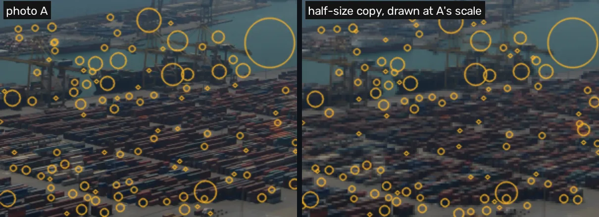
The sizes are right for nearly every point found in place. Requiring the two sizes to agree within a quarter of an octave (an octave is a doubling of size, so a quarter is a factor of 1.19) as well as the position, repeatability at half size goes from 0.295 to 0.284, and at 0.71 from 0.526 to 0.511. Lowe’s own test is looser, a factor of in scale and pixels in position [2].
To see what the size is worth, describe both detectors’ points with SIFT’s 128 numbers (lesson 4), with no direction (every point upright, so only size differs), and match photo A against zoomed copies with the ratio test of lesson 5, which keeps a match only when its nearest candidate is closer than the second nearest by a set margin. A match is correct within 3 px of where the zoom sends the point:
| zoom | Harris, every patch 8 px: correct of matches | SIFT, each patch its own size: correct of matches |
|---|---|---|
| 0.71 | 108 of 116 | 518 of 535 |
| 0.5 | 1 of 1 | 294 of 305 |
| 0.35 | 0 of 0 | 144 of 161 |
At 0.71 the fixed patch still overlaps enough to match some corners. At half size it matches one. The SIFT points lose some matches as the photo shrinks, because fewer of them survive at all, and the ones that survive are matched with the same precision, 89 to 97%. This is the property the rest of the unit is built around: SIFT’s scale invariance comes from a size per point that tracks the zoom. The cell runs the 0.5 row on the photo the page serves.
import numpy as np
import cv2

img = cv2.imread("barcelona-a.webp", cv2.IMREAD_GRAYSCALE)
h, w = img.shape

def rotate(im, deg, zoom=1.0):
    M = cv2.getRotationMatrix2D((w / 2, h / 2), deg, zoom)
    c, s = abs(M[0, 0]), abs(M[0, 1])
    W2, H2 = round(h * s + w * c), round(h * c + w * s)
    M[0, 2] += W2 / 2 - w / 2
    M[1, 2] += H2 / 2 - h / 2
    return cv2.warpAffine(im, M, (W2, H2)), M

sift = cv2.SIFT_create()
print(img.shape)(723, 960)
ZOOM = 0.5
small, Mz = rotate(img, 0, ZOOM)

def harris(im, n=1000, size=8.0):
    c = cv2.goodFeaturesToTrack(im, n, 1e-4, 3, useHarrisDetector=True,
                                k=0.04, blockSize=5)
    return [cv2.KeyPoint(float(x), float(y), size) for x, y in c.reshape(-1, 2)]

def sift_points(im, n=1000):
    kps = sorted(sift.detect(im, None), key=lambda k: -k.response)
    seen, out = set(), []
    for k in kps:
        key = (round(k.pt[0], 2), round(k.pt[1], 2), round(k.size, 2))
        if key not in seen:
            seen.add(key)
            k.angle = 0  # upright: this cell tests size, not direction
            out.append(k)
    return out[:n]

def correct_matches(ka, kb):
    ka, da = sift.compute(img, ka)
    kb, db = sift.compute(small, kb)
    good = [m for m, n in cv2.BFMatcher().knnMatch(da, db, k=2)
            if m.distance < 0.75 * n.distance]
    p = np.array([ka[m.queryIdx].pt for m in good]).reshape(-1, 2)
    q = np.array([kb[m.trainIdx].pt for m in good]).reshape(-1, 2)
    err = np.linalg.norm(p @ Mz[:, :2].T + Mz[:, 2] - q, axis=1)
    return len(good), int((err <= 3).sum())

print("Harris at 8 px:  matches, correct =",
      correct_matches(harris(img), harris(small)))
print("SIFT, own size:  matches, correct =",
correct_matches(sift_points(img), sift_points(small)))Harris at 8 px: matches, correct = (1, 1) SIFT, own size: matches, correct = (287, 270)
On the page this prints 1 correct of 1 for Harris and 270 of 287 for SIFT. Both the cells and the
unit’s experiments shrink the photo with warpAffine; the difference from the table (294 of 305)
comes from the input. The cells read the photo as the page serves it, a WebP copy, and the tables
were measured on the original JPEG resized to the same 960 px.
Distinctive is the other half
A point that comes back in place is useless to a matcher if a hundred other points look like it. The harbour is a hard case: rows of containers of one size and colour, cranes repeated along the quay, windows in a grid. A detector cannot see this, because it judges one point at a time. Distinctiveness belongs to the description and the matching rule: lesson 4 builds the description and measures what each of its parts buys, and lesson 5 shows how SIFT refuses to choose between lookalikes.
Now you try
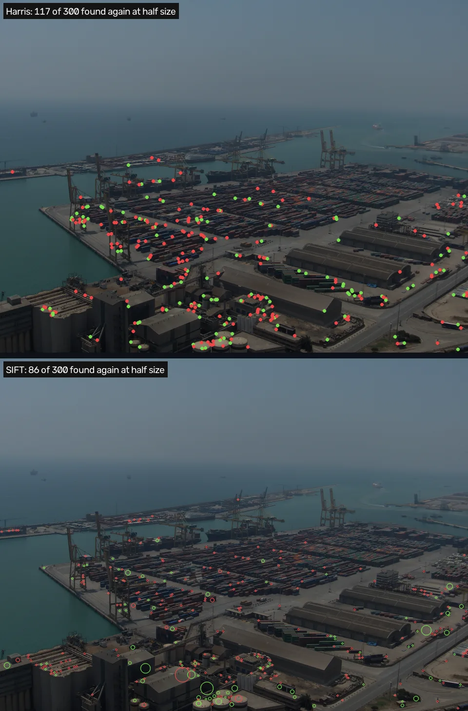
The harbour photo with each detector’s 300 strongest points. Pick a turn and a zoom: the lab redraws the points green where the detector finds them again in the changed copy and red where it does not, and shows the repeatability of those 300 points (0.763 for SIFT at 45°, against 0.729 for the 1,000 strongest in the table) and how many SIFT matches are correct for that change. Set the zoom to 0.5 and switch between Harris and SIFT, then go back to full size and turn the photo to 45°.
How close is this to OpenCV?
OpenCV’s detectors return points; counting the pairs is ours. What can be checked is the geometry
under the count. The first cell repeats the worked example on the served photo, from scratch: the
nearest distances in NumPy and the one-to-one pairing in a loop. The second asks OpenCV’s
BFMatcher, given the point coordinates instead of descriptors, for the same nearest distances.
rot, M = rotate(img, 45)

def strongest(im, n=1000):
    """The n strongest SIFT points, one per position."""
    seen, pts = set(), []
    kps = sorted(sift.detect(im, None), key=lambda k: -k.response)
    for k in kps:
        key = (round(k.pt[0], 2), round(k.pt[1], 2))
        if key not in seen:
            seen.add(key)
            pts.append(k.pt)
    return np.array(pts[:n])

pa, pb = strongest(img), strongest(rot)
qa = pa @ M[:, :2].T + M[:, 2]  # where A's points should land

def inside(p, shape, b=8):
    return ((p[:, 0] >= b) & (p[:, 0] < shape[1] - b)
            & (p[:, 1] >= b) & (p[:, 1] < shape[0] - b))

Mi = cv2.invertAffineTransform(M)
back = pb @ Mi[:, :2].T + Mi[:, 2]
qa, pb = qa[inside(qa, rot.shape)], pb[inside(back, img.shape)]

d = np.linalg.norm(qa[:, None] - pb[None], axis=2)
used, hits = set(), 0
for i in np.argsort(d.min(axis=1)):
    for j in np.argsort(d[i])[:3]:
        if d[i, j] > 1.5:
            break
        if j not in used:
            used.add(j)
            hits += 1
            break
na, nb = len(qa), len(pb)
print(f"{hits} repeated of min({na}, {nb})")
print(f"repeatability {hits / min(na, nb):.3f}")673 repeated of min(1000, 935) repeatability 0.720
bf = cv2.BFMatcher(cv2.NORM_L2)
m = bf.match(qa.astype(np.float32), pb.astype(np.float32))
d_cv = np.array([x.distance for x in m])
print("largest difference in nearest distance:",
      f"{np.abs(d_cv - d.min(axis=1)).max():.2e} px")
print("points with a neighbour within 1.5 px:",
int((d_cv <= 1.5).sum()), " one-to-one:", hits)largest difference in nearest distance: 5.73e-05 px points with a neighbour within 1.5 px: 677 one-to-one: 673
On the page: 673 pairs of min(1000, 935), a repeatability of 0.720 against the worked example’s 0.729, and the largest difference in nearest distance is 5.73e-05 px. The distances agree to float32 rounding. The two counts, 677 and 673, differ by the points of A that have a neighbour within 1.5 px already claimed by a closer point of A: counting “any neighbour within the tolerance” would credit both, and the one-to-one rule credits one.
In the wild
The same measurement on a different photograph: view 1 of the Middlebury templeRing set, a plaster temple on a black background at 640×480 [5], with the 500 strongest points of each detector.
| change | Harris | SIFT | SIFT, with size |
|---|---|---|---|
| turn 45° | 0.715 | 0.796 | 0.780 |
| zoom out to 0.5 | 0.427 | 0.738 | 0.713 |
What it means: on the temple, SIFT comes back far more often at half size, 0.738 against 0.427, where on the harbour Harris led by 0.363 to 0.295. The two photos disagree about which detector repeats better in place, and agree on what matters for matching: SIFT’s sizes are right for almost every point it finds again (0.738 to 0.713 here). I did not test why the temple favours SIFT; the plaster’s rounded, blob-like texture is a guess.
Where this breaks
One number hides two choices. The tolerance and the number of points kept change the ranking of two detectors (the half-size table above). Report both, or report a curve.
Turns and zooms of one photo are the easy case. The copies here keep every pixel’s lighting and viewpoint. A second camera position changes what is hidden behind what, which no 2-D warp reproduces; lesson 5 measures the real pair and a walk around the temple.
SIFT loses points in the dark. Darkening photo A to 0.7, 0.4 and 0.2 of its brightness leaves SIFT with 1,992, 426 and 8 of its 2,897 distinct points. The points that remain come back in place (0.97, 0.962 and 1.0), so the loss is in how many are found: SIFT drops any point whose contrast is below a fixed threshold (lesson 3). Harris here keeps corners whose strength is a fraction of the strongest one in the same photo [7], and repeats 0.993, 0.983 and 0.971 of them.
Noise costs SIFT more than Harris. With σ 8 grey levels of noise, 0.643 against 0.822. A blur of σ 2 px leaves both near 0.38, and SIFT keeps 698 points in the common region instead of 1,000.
A point found again still has to be matched. Every number above counts points found again. A match also needs a description of each point and a rule for which pairs to trust, which the next lessons build.
What this means for your pipeline
- Comparing detectors: state the tolerance and the point count. At half size, Harris leads at 1.5 px (0.363 against 0.295) and SIFT at 1.0 px (0.286 against 0.166).
- Photos at different zooms: use a detector that gives each point a size. Across a 2× zoom, points described at their own size gave 294 correct matches and fixed 8 px patches gave 1.
- Dim photos: expect SIFT to find far fewer points. At 0.4 of the brightness it kept 426 of 2,897; Harris, whose threshold is relative to the strongest corner, still repeated 0.983.
- Noisy photos: SIFT’s points repeat less than Harris’s, 0.643 against 0.822 at σ 8 grey levels.
Exercises
- One point, one partner. Write
one_to_one(d, tol): given a distance matrixd(rows are points of A, columns points of B), pair rows in order of their nearest distance, give each row the nearest column withintolthat no row has taken, and return the number of pairs. The starter counts rows with any neighbour withintol, which credits two rows for one column.
import numpy as np

def one_to_one(d, tol):
    return int((d.min(axis=1) <= tol).sum())  # credits shared partners

print(one_to_one(np.array([[0.5, 3.0], [0.8, 2.0]]), 1.5))
print(one_to_one(np.array([[0.5, 3.0], [3.0, 0.8]]), 1.5))- Predict, then run. In the
repeatcell, turn the photo by 90° instead of 45°. Will repeatability go up or down, and by how much? - Break it. In the
payoffcell, setZOOM = 0.71. Before running, guess how many correct matches the 8 px Harris patches recover now that the zoom is milder.
What you should see
Answer 1 is the solution cell in section 2 of the unit notebook, sift.ipynb. Answers 2 and 3
come from running the modified cells on this page (OpenCV 4.11) and the same modified cells on
OpenCV 5.0, on the same served photo; where the two differ, both are given.
1,2and0. In the first matrix both rows want column 0, and the second row gets nothing, because its other column is 2.0 px away. In the second they want different columns. The starter prints2for the first matrix.- Up, from 0.720 to 0.948 (938 pairs of min(989, 989)) on both versions: a 90° turn moves every pixel to another pixel without resampling, so the detector sees the same numbers. The table gives 0.954.
- Over a hundred: 116 correct of 123 on the page, 117 of 123 on OpenCV 5.0. SIFT gets 485 of 502 and 480 of 494. The table’s 108 of 116 was measured on the original JPEG, not the served WebP, which is enough to move the count.
Check yourself
Four questions on this lesson. Pick an answer to see why it is right or wrong.
Why does the repeatability count divide by the smaller of the two point counts, min(nA, nB)?
Only points both photos can see are counted, and each point of B is used once, so the number of pairs can never exceed the smaller count.
On the harbour photo at half size, Harris corners repeat at 0.363 and SIFT points at 0.295 with a 1.5 px tolerance. What happens at 1.0 px?
SIFT places each point to a fraction of a pixel, so a tight tolerance favours it. The ranking of two detectors moves with the tolerance, which is why a repeatability number must state it.
Described upright and matched against a half-size copy, Harris points with one fixed 8 px patch give 1 correct match. SIFT points give 294. What makes the difference?
Both were described with the same 128 numbers and matched with the same rule. A fixed 8 px patch in the half-size copy covers twice as much harbour as in the original, so the descriptions no longer agree.
Darkening the photo to 0.4 of its brightness leaves SIFT with 426 of its 2,897 points. How often do those 426 come back in place?
SIFT drops every point whose contrast falls below a fixed threshold, so a dark photo gives fewer points, and the ones it keeps are still found in place.
Next
Lesson 2 shows where the size of a SIFT point comes from: blurring the photo at many sizes and finding, for each point, the blur at which it answers most strongly.
Run it: every code block on this page has a cell in the unit’s notebook, open it in Colab.
Further reading
- Schmid, Mohr and Bauckhage [1], for the definition of repeatability used here and a comparison of the detectors of their time under turns, zooms, light and noise.
- Szeliski §7.1.1 “Feature detectors” [3], for the detectors SIFT is one of and the repeatability criterion in a textbook’s words.
- Corners: the structure tensor, for the one-photo test behind the Harris column, with a lab on a real photo.
References
[1] Schmid, C., Mohr, R., & Bauckhage, C. (2000). Evaluation of Interest Point Detectors. International Journal of Computer Vision, 37(2), 151–172. doi:10.1023/A:1008199403446, §3.1 “Repeatability criterion” (the rate over the common part of the two images; author’s manuscript, HAL inria-00548302).
[2] Lowe, D. G. (2004). Distinctive Image Features from Scale-Invariant Keypoints. International Journal of Computer Vision, 60(2), 91–110, §3.2 “Frequency of sampling in scale” (a matching scale is “within a factor of √2 of the correct scale”, a matching location “within σ pixels”). doi:10.1023/B:VISI.0000029664.99615.94
[3] Szeliski, R. (2022). Computer Vision: Algorithms and Applications (2nd ed.), §7.1.1 “Feature detectors”, p. 422, and its paragraph “Measuring repeatability”, p. 428. Springer. Free PDF
[4] Harris, C., & Stephens, M. (1988). A Combined Corner and Edge Detector. Proceedings of the Alvey Vision Conference 1988. doi:10.5244/C.2.23
[5] Seitz, S. M., Curless, B., Diebel, J., Scharstein, D., & Szeliski, R. (2006). A Comparison and Evaluation of Multi-View Stereo Reconstruction Algorithms. CVPR 2006, pp. 519–528. doi:10.1109/CVPR.2006.19. The Middlebury multi-view datasets: vision.middlebury.edu/mview
[6] Pap3rinik. BarcelonaHarbour1.jpg. Wikimedia Commons, public domain. commons.wikimedia.org

[7] OpenCV 4.11.0 source, modules/imgproc/src/featureselect.cpp, goodFeaturesToTrack: corners below maxVal*qualityLevel are zeroed (line 416), so the threshold is a fraction of the best corner’s measure, commit 31b0eee.