
Before this unit: Edge detection
Scale Space and the Difference of Gaussians
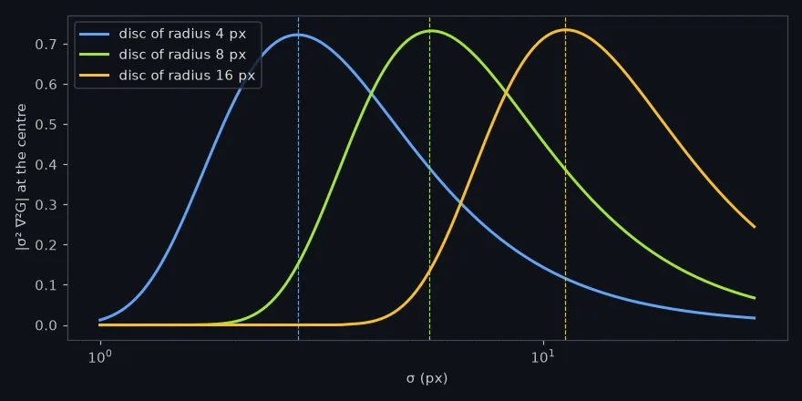
Scale space is a stack of copies of a photo, each blurred a little more, which lets a detector find features of every size and say how big each one is. Discs of radius 4, 8 and 16 px answer most strongly at a blur of 2.77, 5.61 and 11.34 px, close to r/√2; subtracting neighbouring blurs reproduces the scale-normalized Laplacian with a correlation of 0.99; and on a harbour photo SIFT's 9 octaves give each point a size that halves when the photo does.

Scale space is a stack of copies of one photo, each blurred a little more than the one before, and it lets a computer look for features of every size at once and say how big each one is. In the animation below, the matches keep finding the same harbour while the copy on the right shrinks to half its size: that works because each point was found at a size, and the size shrinks with the photo.
The matcher in the animation is SIFT, and every match it draws goes through six steps:
- Blur at many sizes and subtract neighbouring blurs, so features of every size stand out. This lesson.
- Keep the extrema: points brighter or darker than their 26 neighbours in position and blur (lesson 3).
- Refine each point to a fraction of a pixel and drop the weak and edge-like ones (lesson 3).
- Give each point a direction from its strongest gradients (lesson 3).
- Describe it with 128 numbers (lesson 4).
- Match, keeping only pairs whose best candidate is much closer than the second best (lesson 5).
You have met it in:
- Matching photos taken at different zooms, in panoramas, photo search and 3-D reconstruction, where the same window can be a few pixels across in one shot and dozens in the next.
- Blob counters for cells under a microscope or stars in a telescope image, which use the same blurred-and-subtracted images to find round things of every size.
- Image pyramids, the halved copies that map viewers and zoomable photo viewers load at each zoom level, and that multi-scale object detectors run on.
A feature has a size, and the way to find it at any size is to blur the photo step by step and note the blur at which it answers most strongly. Discs of radius 4, 8 and 16 px answer most strongly at a blur of 2.77, 5.61 and 11.34 px, close to (2.83, 5.66 and 11.31). SIFT builds this as 45 subtracted images in 9 octaves (an octave is one doubling of the blur) for the 960×723 harbour photo, and across a zoom to half size the points come back with a median 0.499 of their size.
Where we are
Lesson 2 of SIFT: step 1 of the unit’s pipeline, blurring the photo at many sizes and subtracting neighbouring blurs. Lesson 1 showed that the size SIFT gives each point is what lets it match across a zoom. This lesson builds the stack the sizes come from; lesson 3 finds the points in it. The blur is the Gaussian of 2-D convolution, and the second derivative is the Laplacian of unit 3.1’s Laplacian lesson.
One window finds one size
Every detector looks at a photo through a window of some size. The corner test of unit 3.1 uses a fixed one, and so does a blob detector that blurs the photo once. Something much larger than the window looks flat or like an edge from inside it; something much smaller is averaged away.
Bright discs on a black background make this measurable. A standard blob detector blurs with a
Gaussian of width (in pixels), takes the Laplacian (the sum of the second derivatives in
and , large where the brightness has a peak or a dip), and reads it at the disc’s centre.
Fix at 5.61 px, the value that suits a disc of radius 8 px, and the disc of radius 4 px
answers at about half of its best, the disc of radius 16 px at about a fifth (the discs cell below
prints both). A detector with one sees one size of disc well.
Blur and compare
The fix is to try every and keep, for each spot, the one at which it answers most. The photo becomes a stack : the photo blurred with a Gaussian of width , for a range of . This stack is scale space, a 3-D block with two axes of position and one of blur, and under reasonable assumptions the Gaussian is the only blur that can build it, a result Lowe cites from Koenderink and Lindeberg [2]. Szeliski describes the same search over position and scale as the standard way to make a detector work at every size [3].
Comparing answers across the stack needs one correction. Blurring flattens everything, so the raw Laplacian shrinks as grows and the smallest would always win. Multiplying by undoes that; Lindeberg showed this scale normalization is what makes the answers at different comparable, so that the best follows the size of the structure in pixels, and doubles when a zoom doubles it [1], and the resulting is the scale-normalized Laplacian of Gaussian. For a disc of radius , its response at the centre is largest near , which the worked example measures.
Subtract instead of differentiating
Computing the Laplacian on every blurred copy is a second filter per level. Lowe’s way out is to subtract neighbouring blurs [2]. If two copies differ in blur by a constant factor ,
is the difference of Gaussians (DoG), and from the heat equation (blurring is heat spreading through the image)
In Lowe’s words, “when the difference-of-Gaussian function has scales differing by a constant factor it already incorporates the σ² scale normalization required for the scale-invariant Laplacian” [2]. The blurred copies are needed anyway, so each DoG costs one subtraction, and the constant is the same for every level, so it moves no peak.
How good is the approximation on a real photo? On the harbour photo, the DoG level at with SIFT’s , against at the same , pixel by pixel: correlation 0.9895, and the difference is 18% of the DoG’s size (its norm, relative). The two pick out the same structures; the difference is a slightly different weighting of fine and coarse detail, since spans to while the Laplacian sits at one .
Octaves: stop blurring, start shrinking
Blurring to large costs more as the kernel grows, and once has doubled, half the pixels carry no detail the blur has not already removed. So the stack is built in octaves, one per doubling of : blur in steps of until has doubled, then keep every second pixel of that copy and start the next octave from it, at the same relative blur and a quarter of the pixels [2].
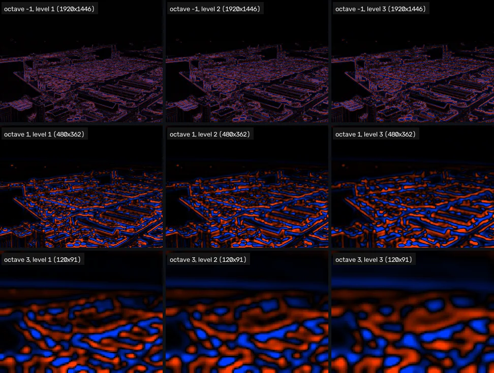
SIFT takes three searchable levels per octave, the number at which Lowe measured the highest repeatability [2], so and each octave holds Gaussian copies and 5 DoG images. It also starts from the photo doubled in size, so that features smaller than the starting blur still have pixels to be found in: Lowe writes that “the image doubling increases the number of stable keypoints by almost a factor of 4” [2].
What the stack gives each point: a size
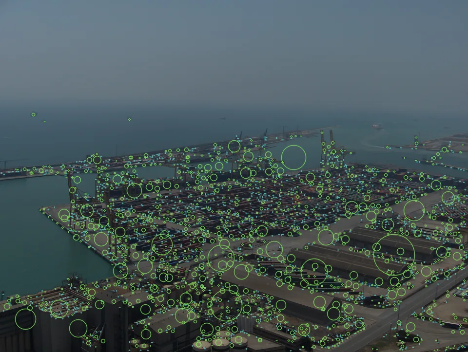
Lesson 3 finds the points of the stack that beat their neighbours in position and in blur. Each one’s blur, scaled back to the photo, is its size. On the harbour photo the 2,897 distinct points range from 1.8 to 84.3 px, with a median of 2.99 px: most are small, and a few span whole buildings.
| octave | −1 (doubled base) | 0 | 1 | 2 | 3 | 4 |
|---|---|---|---|---|---|---|
| points | 1,840 | 753 | 219 | 67 | 16 | 2 |
Almost two in three points, 1,840 of 2,897 (64%), come from the doubled base: structures too small to be found at the photo’s own resolution.
The test of a size is whether it follows the zoom. Shrink the photo, match it against the original (the points that land within 3 px of the right place), and divide each point’s size in the copy by its size in the original:
| zoom | correct matches | size ratio, median | 5th to 95th percentile |
|---|---|---|---|
| 0.71 | 1,166 | 0.713 | 0.658 to 0.786 |
| 0.5 | 674 | 0.499 | 0.464 to 0.542 |
| 0.35 | 270 | 0.349 | 0.311 to 0.389 |
The sizes come back at the zoom: nine points in ten within about 7 to 11% of it, either way. That is what lesson 1’s matches across a zoom relied on: a size measured from the photo, so a description taken at that size covers the same piece of harbour in both.
Now you try
Five bright discs of radius 2, 3, 5, 8 and 12 px, and one σ slider (0.6 to 12). The lab blurs the scene at σ and at 1.6σ, subtracts, and reads the DoG at each disc’s centre; a disc lights up while σ sits near its own peak. Sweep σ and watch the discs light up from smallest to largest. The readout puts the peak near 0.48 of the radius instead of 0.71. The lab differs from the cells below in three ways that each move the peak: its two blurs are 1.6 apart, wider than SIFT’s 1.26, the level is labelled with the smaller of the two, and it approximates the Gaussian with box blurs to run live. I did not measure how much of the gap each one accounts for.
How close is this to OpenCV?
Three checks on the photo the page serves. First, a Gaussian blur built in NumPy (a 1-D kernel run
along the rows, then the columns) against cv2.GaussianBlur. Second, the DoG against
on the same photo, at the and of the worked numbers above.
Third, the disc sweep at three radii.
import numpy as np
import cv2

img = cv2.imread("barcelona-a.webp", cv2.IMREAD_GRAYSCALE)
img = img.astype(np.float32)

def gauss_kernel(sigma):
    r = int(np.ceil(3 * sigma))
    x = np.arange(-r, r + 1)
    g = np.exp(-x**2 / (2 * sigma**2))
    return (g / g.sum()).astype(np.float32)

def blur(im, sigma):
    """Separable Gaussian: rows, then columns, mirrored borders."""
    g = gauss_kernel(sigma)
    r = len(g) // 2
    p = np.pad(im, r, mode="reflect")
    rows = sum(g[i] * p[:, i:i + im.shape[1]] for i in range(len(g)))
    return sum(g[i] * rows[i:i + im.shape[0], :] for i in range(len(g)))

sigma = 2.54
mine = blur(img, sigma)
ref = cv2.GaussianBlur(img, (0, 0), sigma, borderType=cv2.BORDER_REFLECT_101)
k = 2 * int(np.ceil(3 * sigma)) + 1
ref_same = cv2.GaussianBlur(img, (k, k), sigma, borderType=cv2.BORDER_REFLECT_101)
print("largest difference, same kernel width:",
      f"{np.abs(mine - ref_same).max():.4f} grey levels")
print("largest difference, OpenCV's own width:",
f"{np.abs(mine - ref).max():.4f} grey levels")largest difference, same kernel width: 0.0001 grey levels largest difference, OpenCV's own width: 0.1632 grey levels
With a kernel of the same width, ±3σ, the two agree to 0.0001 of a grey level, the rounding of float32 sums. Left to choose the width itself, OpenCV goes out to ±4σ for a floating-point image [6], and the extra tails move pixels by up to 0.16 of a grey level: the two blurs are the same filter cut off at different places.
k = 2 ** (1 / 3)  # three levels per octave
d = blur(img, k * sigma) - blur(img, sigma)
lap = cv2.Laplacian(blur(img, sigma), cv2.CV_32F, ksize=1)
approx = (k - 1) * sigma**2 * lap

m = (slice(20, -20), slice(20, -20))  # leave the borders out
a, b = d[m].ravel(), approx[m].ravel()
print(f"k = {k:.4f}, sigma = {sigma}")
print(f"correlation {np.corrcoef(a, b)[0, 1]:.4f}")
print(f"relative residual {np.linalg.norm(a - b) / np.linalg.norm(a):.3f}")k = 1.2599, sigma = 2.54 correlation 0.9897 relative residual 0.178
The cell prints a correlation of 0.9897 and a relative residual of 0.178. The figures above, 0.9895 and 0.18, come from SIFT’s own pyramid, which blurs the doubled photo step by step instead of blurring the photo once per ; the two routes agree to the third decimal.
sigmas = np.geomspace(1, 40, 200)

def disc_response(r, s):
    disc = np.zeros((257, 257), np.float32)
    cv2.circle(disc, (128, 128), r, 1.0, -1, lineType=cv2.LINE_AA)
    g = cv2.GaussianBlur(disc, (0, 0), s)
    return abs(s**2 * cv2.Laplacian(g, cv2.CV_32F, ksize=1)[128, 128])

for r in (4, 8, 16):
    resp = [disc_response(r, s) for s in sigmas]
    best = sigmas[int(np.argmax(resp))]
    fixed = disc_response(r, 5.61) / max(resp)
    print(f"radius {r:2d}: best sigma {best:5.2f}, r/sqrt(2) "
f"{r / np.sqrt(2):5.2f}, at sigma 5.61: {fixed:.0%} of its best")radius 4: best sigma 2.77, r/sqrt(2) 2.83, at sigma 5.61: 53% of its best radius 8: best sigma 5.61, r/sqrt(2) 5.66, at sigma 5.61: 100% of its best radius 16: best sigma 11.34, r/sqrt(2) 11.31, at sigma 5.61: 20% of its best
It prints the worked example’s three best values, 2.77, 5.61 and 11.34, and the cost of a fixed blur: at the 4 px disc answers at 53% of its best and the 16 px disc at 20%.
In the wild
View 1 of the Middlebury templeRing set [4] is 640×480. Doubled, its smaller side is 960, and : the same nine octaves as the harbour, from a photo with less than half the pixels. Its 683 distinct SIFT points spread over the octaves much as the harbour’s do, 391 of them (57%) from the doubled base, and across a zoom to half size its correctly matched points come back with a median size ratio of 0.499 (5th to 95th percentile 0.448 to 0.530), the same as the harbour’s 0.499.
What it means: on two very different photos, a plaster temple on black and a harbour full of containers, the sizes follow the zoom the same way, to three decimals at the median. Two photos do not show that this holds for every scene.
Where this breaks
Scale is not the only change. The stack copes with a zoom, the same picture made larger or smaller. A camera that tilts squeezes a round blob into an ellipse, and no single fits an ellipse; the descriptor of lesson 4 absorbs a little of that, and the real pair in lesson 5 shows where it stops.
The sizes are in steps. Three levels per octave means neighbouring levels differ by 26% in blur; the true size between them is found by fitting a curve across levels, which is lesson 3’s job. The tracking table’s spread, about 7 to 11% either way, is what remains after that fit.
The photo arrives already blurred. The camera’s own blur and the JPEG’s smoothing set the starting blur. SIFT assumes the photo arrives with a blur of 0.5 px [2]; a soft photo shifts every size a little and loses the smallest points.
Most points are tiny. The median point is 3 px across and 64% come from the doubled base. Those are the first to disappear under blur, noise or compression, which may be part of why SIFT’s repeatability fell to 0.643 under noise in lesson 1, against 0.822 for Harris.
What this means for your pipeline
- Matching across zooms needs a size per point, and the size comes from the blur at which the point answers most: on the harbour, sizes come back at a median 0.499 after halving the photo.
- Most of SIFT’s points are tiny: 64% come from the doubled base and the median is 2.99 px. A soft, noisy or heavily compressed photo loses those first.
- Bigger photos get deeper pyramids: 9 octaves for 960×723, 12 for 4000×3000, with 5 DoG images each.
- The DoG approximates the Laplacian closely at SIFT’s : correlation 0.9895, falling to 0.9070 at .
Exercises
- Count the octaves. Write
n_octaves(w, h)from the worked example: double the smaller side, take , subtract 2, round, add 1.
import numpy as np

def n_octaves(w, h):
    return 0  # round(log2(2 * smaller side) - 2) + 1

print(n_octaves(960, 723), n_octaves(640, 480), n_octaves(4000, 3000))- Predict, then run. In the
discscell, add a disc of radius 32 px. At what will it answer most? - Break it. In the
dogcell, setk = 2. Lowe found the approximation still works for detection at ; guess what happens to the correlation at 2.
What you should see
Answer 1 is the solution cell in section 3 of the unit notebook, sift.ipynb. Answers 2 and 3
come from running the modified cells on this page (OpenCV 4.11) and the same modified cells on
OpenCV 5.0, on the same served photo; where the two differ, both are given.
n_octaves(960, 723)is 9,n_octaves(640, 480)is 9 andn_octaves(4000, 3000)is 12: a 12-megapixel photo gets three more octaves than the harbour. Its smaller side is 4.15 times the harbour’s, about 2.05 doublings; the third extra octave comes from the rounding, since 8.498 rounds down to 8 and 10.55 rounds up to 11.- At 22.52, against , on both versions. At the 32 px disc prints 0% of its best: a blur that suits an 8 px disc does not see it at all.
- The correlation falls from 0.9897 to 0.9070 and the relative residual rises from 0.178 to 0.655, on both versions. The DoG still marks the same structures, which is why detection survives, and its values are no longer a good stand-in for the Laplacian’s.
Check yourself
Four questions on this lesson. Pick an answer to see why it is right or wrong.
A blob detector blurs once, at σ = 5.61 px, the blur that suits a disc of radius 8 px. How strongly does a disc of radius 16 px answer?
One blur suits one size. The 16 px disc answers most at σ = 11.34; at 5.61 it gives 20% of that, and the 4 px disc 53% of its best.
Why is the Laplacian multiplied by σ² before responses at different blurs are compared?
The raw Laplacian shrinks as σ grows, so the smallest σ would always win. Lindeberg showed that the σ² normalization makes answers at different σ comparable, so the best σ follows the size of the structure in pixels.
On the harbour photo, how well does the difference of two Gaussians (k = 1.26) match (k − 1)σ²∇²G at σ = 2.54?
The heat equation gives G(kσ) − G(σ) ≈ (k − 1)σ²∇²G. On the photo the two correlate at 0.9895; at k = 2 the correlation falls to 0.907.
The harbour photo is 960×723. Why does SIFT search 9 octaves and 27 DoG levels on it?
round(log2 1446 − 2) + 1 = 9 octaves for the 1920×1446 doubled base, and only the middle three of each octave’s five DoG images have a level above and below to compare with.
Next
Lesson 3 searches the 27 DoG levels for points that beat all 26 of their neighbours, places each one between pixels and between levels, and throws away the weak ones and the ones that sit on edges.
Run it: every code block on this page has a cell in the unit’s notebook, open it in Colab.
Further reading
- Lowe’s §3 [2], “Detection of scale-space extrema”, for the pyramid’s construction and the experiments behind three levels per octave and σ = 1.6.
- Lindeberg [1], for scale selection itself: why the normalization is σ², and how the best scale relates to a blob’s size.
- Szeliski §7.1.1 “Feature detectors” [3], for scale space among the other ways to make a detector work at many sizes.
- The Laplacian, zero-crossings and LoG, for the Laplacian of Gaussian as an edge detector, the use it had before SIFT.
References
[1] Lindeberg, T. (1998). Feature Detection with Automatic Scale Selection. International Journal of Computer Vision, 30(2), 79–116. doi:10.1023/A:1008045108935, §3 “Normalized derivatives and intuitive idea for scale selection” (the γ-normalized derivative, eq. 9) and §5.1, Example 1 (a Gaussian blob’s Laplacian peaks at the blob’s own scale, eq. 37). Author’s copy: KTH technical report ISRN KTH/NA/P–96/18–SE, revised 1998.
[2] Lowe, D. G. (2004). Distinctive Image Features from Scale-Invariant Keypoints. International Journal of Computer Vision, 60(2), 91–110, §3 “Detection of scale-space extrema” (equation (1), Figure 1, the (k − 1)σ²∇²G approximation), §3.2 “Frequency of sampling in scale” (three scales per octave) and §3.3 “Frequency of sampling in the spatial domain” (σ = 1.6, the doubled image, an assumed blur of 0.5). doi:10.1023/B:VISI.0000029664.99615.94
[3] Szeliski, R. (2022). Computer Vision: Algorithms and Applications (2nd ed.), §7.1.1 “Feature detectors”, p. 422, and its paragraph “Scale invariance”, pp. 428–429. Springer. Free PDF
[4] Seitz, S. M., Curless, B., Diebel, J., Scharstein, D., & Szeliski, R. (2006). A Comparison and Evaluation of Multi-View Stereo Reconstruction Algorithms. CVPR 2006, pp. 519–528. doi:10.1109/CVPR.2006.19. The Middlebury multi-view datasets: vision.middlebury.edu/mview
[5] Pap3rinik. BarcelonaHarbour1.jpg. Wikimedia Commons, public domain. commons.wikimedia.org

[6] OpenCV 4.11.0 source, modules/imgproc/src/smooth.dispatch.cpp: with ksize (0, 0), the Gaussian kernel reaches ±4σ for a floating-point image and ±3σ for an 8-bit one. The rule is ksize = cvRound(sigma*(depth == CV_8U ? 3 : 4)*2 + 1)|1 (lines 289 and 291), commit 31b0eee.