How SIFT Finds Keypoints: Extrema, Refinement, Orientation

SIFT’s detector looks through a photo at every size at once and keeps only the points it expects to find again in another photo of the same scene: small blobs and corners, each with a position, a size and a direction. The animation shows what those points are for: SIFT finds them on two photos of Barcelona harbour, pairs each with its most similar point in the other photo, and keeps the pairs it trusts.

1. Blur the photo at many sizes and subtract neighbouring blurs, so that every size of blob gets a layer where it stands out (lesson 2).
2. Keep the extrema: the points brighter or darker than all 26 neighbours around them in position and in blur.
3. Refine and test: move each one to where a smooth fit puts the peak, then drop the ones too faint to survive noise and the ones that lie along an edge.
4. Give it a direction: the most common gradient direction around it, so that the next step can describe it the same way however the photo is turned.
5. Describe each point with 128 numbers (lesson 4).
6. Match the numbers between photos (lesson 5).

You have met these points in:

• Panorama apps, which find them in neighbouring photos before stitching (image alignment does it with this pair).
• 3-D reconstruction from photos, which triangulates them (structure from motion).
• Visual localisation and AR, which recognise a place by the points it has seen before.
• Image search by landmark, which compared bags of such points before learned features.

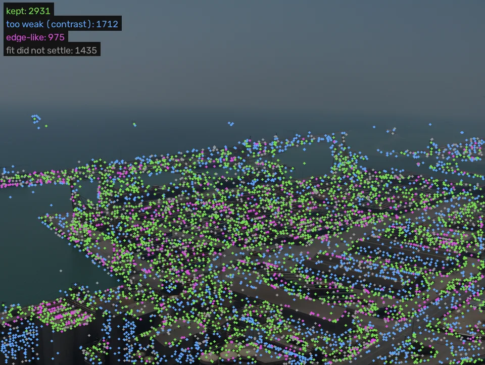
Most of what the first test finds is thrown away, and each test removes a different kind of bad point. On photo A, the detector built from scratch with OpenCV’s constants finds 7,053 points that beat their 26 neighbours; the fit never settles for 1,435, 1,712 are too faint and 975 sit on edges, leaving 2,896 distinct points and 3,510 keypoints once each gets its directions. It finds 99.63% of OpenCV’s 3,471 keypoints within 0.1 px.

Where we are

Lesson 3 of SIFT, steps 2 to 4 of its pipeline. Lesson 1 set the criterion: a good keypoint is found again after the camera moves, at the same place and size. Lesson 2 built the stack this lesson searches: the photo blurred at sizes 2^(1/3) apart, and the difference of each neighbouring pair (the DoG, difference of Gaussians), which is strongest on blobs of the matching size. The output here, a list of points with a position, a size and a direction, is what lesson 4 describes. The detector is Lowe’s [1], and Szeliski places it among the other detectors in §7.1.1 [2].

Candidates: beat all 26 neighbours

A blob of a given size makes a peak in one layer of the DoG stack, at its centre. So the candidates are the samples that are larger than every neighbour, or smaller than every neighbour: the 8 around them in their own layer and the 9 in each layer above and below. That compares each sample with 26 others, in position and in size at once, and a sample that wins is a blob centre at its own size.

Of the 5 DoG layers per octave, the 3 in the middle have a layer on both sides, so those are the ones searched. OpenCV also skips the 5 pixels next to the border and any sample within one grey level of zero, a floor of $\lfloor 0.5 \times 0.04 / 3 \times 255 \rfloor = 1$ that only saves time [3].

On photo A that leaves 7,053 candidates over 9 octaves. Many of them are wrong in one of three ways, and the next three steps catch one each.

Refine: placing the peak between samples

A candidate is a sample of the grid, and the peak of a blob rarely falls on one. Lowe adopted Brown’s fix [1]: fit a smooth quadratic to the DoG values around the sample, in $x$, $y$ and blur, and move to the top of that quadratic. The fit uses the first and second differences of the 3×3×3 neighbourhood, and its peak sits at an offset

from the sample. If the offset is more than half a sample in any direction, the peak belongs to a neighbouring sample: the fit moves there and runs again, up to 5 times in OpenCV. A candidate whose fit keeps moving, or walks off the octave, is dropped.

On photo A the fit never settles for 1,435 candidates (20%). For the keypoints that remain, the median move is 0.224 px in the photo’s own pixels and 95% move less than 0.885 px: small, but not small next to the 3 px within which lesson 5 calls a match correct.

Drop the faint ones: the contrast test

The quadratic also gives the DoG value at its peak, $|D(\hat{\mathbf{x}})|$, which is how strongly the blob stands out from its surroundings. A faint peak can come from noise, and the next photo’s noise will put it somewhere else. Lowe dropped peaks below 0.03 on a 0 to 1 scale [1]; OpenCV’s default is $0.04 / 3 \approx$ 0.0133, the contrastThreshold divided by the 3 layers per octave [3].

This removes 1,712 candidates on photo A, more than any other test. Many are the blue dots along the hazy horizon and on the water above: haze has little contrast, and its DoG peaks are small.

Drop the edge-like ones: the edge test

A DoG layer also responds strongly along an edge, such as the line where a quay meets the water. Seen from the side, the edge is a clear peak; along it, every position looks the same. That is the long quay edge of lesson 1: the detector can say “on the edge” but not “here on the edge”, so in the next photo the point slides along it and the match lands somewhere else.

The shape of the peak tells the two apart. The 2×2 Hessian $H$ of the DoG layer, its second differences in $x$ and $y$, has two eigenvalues: how sharply the layer curves in the steepest and the flattest direction. A blob curves about equally both ways; an edge curves a lot across and almost not at all along. Lowe tests the ratio without computing the eigenvalues, borrowing the trick of Harris and Stephens [4]: with $\alpha = r\beta$,

and a point is kept when the left side is below $(r+1)^2/r$ at $r = 10$, that is below $121/10 = 12.1$ [1]. A negative determinant means the layer curves up one way and down the other, a saddle, and is dropped too.

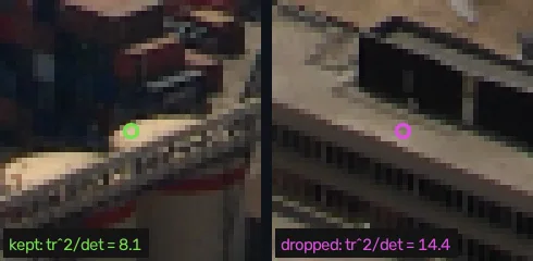
The edge test removes 975 candidates on photo A, the magenta dots along quays and roof lines in the figure above.

Now you try

Every candidate of photo A, with its contrast and its curvature ratio measured once. Move the contrast threshold up and watch the hazy sky empty first; move the edge ratio $r$ down toward 1 and watch the kept points along straight structures turn magenta. At the defaults (0.04 and 10) the counts are those of the from-scratch detector run with OpenCV’s constants: 1,435 unsettled, 1,712 too weak, 975 edge-like, 2,931 kept.

The 2,931 survivors are not all distinct: when two neighbouring candidates refine to the same sample, they become one point. 35 merge that way, leaving 2,896 points.

A direction for every point

Lesson 4 describes the neighbourhood of each point in a grid of gradient directions. If that grid stayed fixed to the photo’s axes, turning the camera would turn every direction in it and the description would change. So each point gets its own direction first, and the grid is laid along it.

The direction is the most common gradient direction around the point. OpenCV takes the Gaussian layer at the point’s blur $\sigma$, measures the gradient at every pixel within $4.5\sigma$ of it, and adds each gradient’s strength to one of 36 bins of 10°, weighted by a Gaussian of $1.5\sigma$ around the point [1]. The histogram is smoothed, the tallest bin wins, and a parabola through it and its two neighbours places the peak between bins.

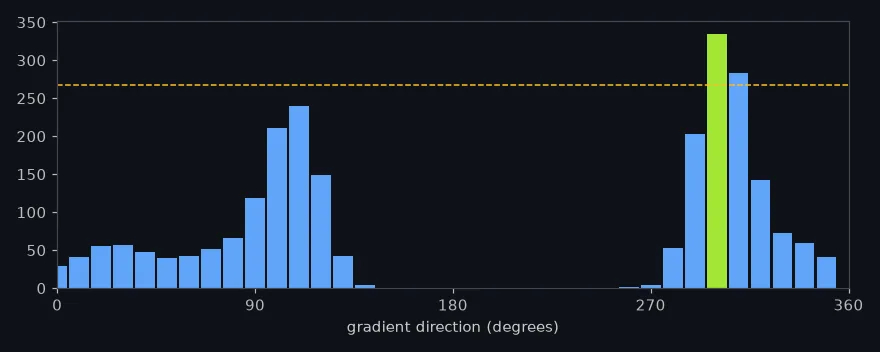
That 80% rule is the last thing the detector does. When a second peak reaches 80% of the first, SIFT makes a copy of the point with the second direction, because either could be the one the next photo picks [1]. On photo A, 572 of the 2,896 points (about one in five) get two or more directions, adding 614 copies: 3,510 keypoints in all. Lowe reports about 15% of points with several directions on his images [1].

How close is this to OpenCV?

The from-scratch detector of the companion repo (features/sift_scratch.py) follows OpenCV’s source step by step, with its constants [3]. On photo A it finds 99.63% of OpenCV’s 3,471 keypoints within 0.1 px, with the same size (median ratio 1.0) and an angle within 0.00021° for 95% of them. It returns 3,510 keypoints to OpenCV’s 3,471. It is also slow: 0.61 s for the photo against 0.036 s for cv2.SIFT, because Python loops over thousands of candidates where OpenCV runs compiled code.

The cells below rebuild one octave, the one at the photo’s own size, and find its candidates. They fetch photo A as the site serves it (a WebP of the same 960×723 photo), so their counts can differ slightly from the companion repo’s.

import numpy as np
import cv2

img = cv2.imread("barcelona-a.webp", cv2.IMREAD_GRAYSCALE)
g = img.astype(np.float32)

# SIFT doubles the photo first (assumed blur 0.5 becomes 1.0)
# and blurs it to 1.6; each level is 2^(1/3) blurrier.
k = 2 ** (1 / 3)
sig = [1.6 * k ** i for i in range(6)]
big = cv2.resize(g, None, fx=2, fy=2, interpolation=cv2.INTER_LINEAR)
big = cv2.GaussianBlur(big, (0, 0), np.sqrt(1.6**2 - 1.0**2))
for i in (1, 2, 3):  # up to twice the start blur ...
    big = cv2.GaussianBlur(big, (0, 0), np.sqrt(sig[i]**2 - sig[i-1]**2))
levels = [big[::2, ::2]]  # ... then halve: the octave at the photo's size
for i in range(1, 6):
    step = np.sqrt(sig[i]**2 - sig[i - 1]**2)
    levels.append(cv2.GaussianBlur(levels[-1], (0, 0), step))
dog = [levels[i + 1] - levels[i] for i in range(5)]

# A point is kept if it beats (or ties) its 26 neighbours
# in x, y and scale, and is more than 1 grey level from 0.
box = np.ones((3, 3), np.uint8)
pts = []
for i in (1, 2, 3):
    cube = np.stack(dog[i - 1:i + 2])
    hi = cv2.dilate(cube.max(axis=0), box)
    lo = cv2.erode(cube.min(axis=0), box)
    v = dog[i]
    hit = ((v > 1) & (v >= hi)) | ((v < -1) & (v <= lo))
    hit[:5] = hit[-5:] = False
    hit[:, :5] = hit[:, -5:] = False
    for r, c in zip(*np.nonzero(hit)):
        pts.append((i, r, c))
print("octave size:", levels[0].shape[::-1])
print("extrema in this octave:", len(pts))

octave size: (960, 723)
extrema in this octave: 1595

cv2.dilate with a 3×3 box replaces each pixel by the largest value around it, so a sample that equals the dilated maximum of the three stacked layers is the largest of its 27. Now the two tests, here at the integer sample without the sub-pixel fit:

# Contrast and edge tests at the integer point (no sub-pixel fit).
keep = 0
weak = edge = 0
for i, r, c in pts:
    d = dog[i]
    if abs(d[r, c]) / 255 * 3 < 0.04:   # contrast test
        weak += 1
        continue
    dxx = d[r, c + 1] + d[r, c - 1] - 2 * d[r, c]
    dyy = d[r + 1, c] + d[r - 1, c] - 2 * d[r, c]
    dxy = (d[r + 1, c + 1] - d[r + 1, c - 1]
           - d[r - 1, c + 1] + d[r - 1, c - 1]) / 4
    tr, det = dxx + dyy, dxx * dyy - dxy ** 2
    if det <= 0 or tr * tr / det >= 11 ** 2 / 10:  # edge test, r = 10
        edge += 1
        continue
    keep += 1
print("too weak:", weak, " edge-like:", edge, " kept:", keep)

too weak: 464  edge-like: 286  kept: 845

The check against OpenCV: every keypoint cv2.SIFT reports in this octave should sit on or next to one of our candidates, since refinement moves a point by about half a sample at most unless it hops to a neighbour.

# How close: OpenCV's keypoints found at this resolution (octave 0)
# against our raw extrema of the same octave.
kps = cv2.SIFT_create().detect(img, None)
octave = [((kp.octave & 255) ^ 128) - 128 for kp in kps]
mine = np.array([(c, r) for i, r, c in pts], np.float32)
theirs = np.array([kp.pt for kp, o in zip(kps, octave) if o == 0],
                  np.float32)
m = cv2.BFMatcher(cv2.NORM_L2).match(theirs, mine)
d = np.array([x.distance for x in m])
print("OpenCV keypoints in octave 0:", len(theirs))
print("within 1 px of one of ours:", f"{(d <= 1).mean():.1%}")
print("within 2 px:", f"{(d <= 2).mean():.1%}")
print("largest distance:", f"{d.max():.2f} px")

OpenCV keypoints in octave 0: 870
within 1 px of one of ours: 99.2%
within 2 px: 100.0%
largest distance: 1.42 px

Of OpenCV’s 870 keypoints at this size, 99.2% sit within 1 px of one of our candidates and all within 2 px: the gaps are the sub-pixel moves of the previous section. OpenCV numbers its octaves from −1, the doubled one, so octave 0 is the photo’s own size. The octave number is packed into the low byte of KeyPoint.octave as a signed value, which is what the ^ 128 line unpacks.

The same tests can be switched off in OpenCV itself. contrastThreshold near zero turns off the contrast test and a huge edgeThreshold the edge test. These counts include the orientation copies:

# OpenCV's route: switch each test off and count what it removes.
def count(**kw):
    return len(cv2.SIFT_create(**kw).detect(img, None))

both = count()
no_contrast = count(contrastThreshold=1e-9)
no_edge = count(edgeThreshold=1e9)
neither = count(contrastThreshold=1e-9, edgeThreshold=1e9)
print("both tests off:", neither)
print("contrast test only:", no_edge)
print("edge test only:", no_contrast)
print("both on (default):", both)

both tests off: 9121
contrast test only: 4327
edge test only: 7473
both on (default): 3492

On this page (OpenCV 4.11) the contrast test alone takes the count from 9,121 to 4,327 and the edge test alone to 7,473 (on OpenCV 5.0: 9,015, 4,326 and 7,365, with 3,491 for both), so on this photo the contrast test removes more, as it did in the from-scratch count above. The two overlap. If they removed different points, both together would leave $9{,}121 - 4{,}794 - 1{,}648 = 2{,}679$; they leave 3,492, so 813 keypoints fail both tests.

In the wild

The same detector on templeR0001, a 640×480 photo of a plaster temple from the Middlebury multi-view dataset [6]: 2,517 candidates; the fit does not settle for 392, 1,100 are too weak and 341 edge-like, leaving 684, which merge into 683 points and 802 keypoints. OpenCV finds 801, and the from-scratch detector finds every one of them within 0.1 px.

What it means: on the temple the contrast test removes 44% of the candidates against 24% on the harbour. The temple stands on a black background, and my guess, which I did not test, is that the background does what the haze does on the harbour: it gives peaks too faint to trust. The harbour has more texture per pixel, and 41% of its candidates survive against the temple’s 27%.

Where this breaks

The thresholds are absolute. The contrast test compares the DoG value with a fixed number, so a darker photo has weaker peaks everywhere. Lesson 1 measured it with OpenCV’s detector: photo A has 2,897 distinct points, 1,992 at 0.7 of its brightness, 426 at 0.4 and 8 at 0.2. A detector you want to work at dusk needs a lower contrastThreshold, and more noise comes with it.

The edge test measures curvature only. A point is kept if it curves within a ratio of 10 both ways. A long blob at the right size, such as a short white car seen from above, passes, and the next photo may place it a pixel or two differently along its length.

One direction per peak, and the peak can flip. A point with two nearly equal directions gets two keypoints; one at 79% of the tallest gets one, and a little noise can make the other direction win in the next photo. The copies are SIFT’s insurance against that, and they cost memory: 614 extra keypoints here.

A small point has a small window. The strongest point on photo A is 2.07 px across, found in the doubled octave. Its direction comes from a window about 9 px across in the photo, and every other sample in it was made up by the doubling’s interpolation.

The candidates come from blur, so blur changes them. Blur the photo and the small blobs disappear from the stack before any test sees them (exercise 3).

What this means for your pipeline

• Dim or hazy photos lose most of their candidates to the contrast test: on photo A it removes 1,712 of 7,053, more than any other step. Lowering contrastThreshold brings points back with more noise among them.
• Points along edges are dropped on purpose: 975 here. A scene made of straight lines (façades, quays, documents) yields fewer SIFT points than its edge count suggests.
• Expect about one point in five to come twice, with two directions: 572 of 2,896 here. Count distinct points when you compare detectors, because the copies inflate keypoint counts.
• Positions are sub-pixel: the fit moves a point by a median 0.224 px, so a tolerance below 1 px is meaningful for SIFT.

Exercises

1. The edge test. Write edge_ok(dxx, dyy, dxy, r=10) that returns True when a point with these second differences passes the edge test. Use the worked example’s two points and a saddle to test it.

def edge_ok(dxx, dyy, dxy, r=10):
    return True  # replace with the test

print(edge_ok(5.2592, 19.0113, 5.2267))   # the compact spot
print(edge_ok(1.0634, 5.0496, -1.6645))   # the straight edge
print(edge_ok(3.0, -2.0, 0.0))       # a saddle

2. Predict, then run. In the cell “Contrast and edge tests, at the sample”, change the edge ratio from $r = 10$ to $r = 5$ (11 ** 2 / 10 becomes 6 ** 2 / 5). How many of the candidates will be edge-like now, and does the contrast count change?
3. Break it. In the first cell, blur the photo by σ = 4 before building the octave (add img = cv2.GaussianBlur(img, (0, 0), 4) after reading it). Guess the number of candidates before running, then run the first two cells.

Next

Lesson 4: the SIFT descriptor takes each keypoint’s position, size and direction and lays a 4×4 grid of gradient histograms over its neighbourhood: 128 numbers that should come out the same in the other photo. The criterion they are scored by is lesson 1’s, and the stack they are found in is lesson 2’s.

Run it: every code block on this page has a cell in the unit’s notebook, open it in Colab.

Further reading

• The source: Lowe 2004 [1], §4 and §4.1, for the sub-pixel fit and the edge test in three pages, with a figure of the same three stages on a small photo (832, 729 and 536 points).
• The book: Szeliski §7.1.1 [2], for SIFT’s detector next to Förstner–Harris and the others, and how detectors are compared.
• The code: OpenCV’s sift.simd.hpp [3], adjustLocalExtrema and calcOrientationHist, which this lesson’s from-scratch version follows line by line.
• Related on CondadosAI: Corner detection is the structure tensor the edge test borrows its trick from, and the Laplacian lesson is the operator the DoG stands in for.

References

[1] Lowe, D. G. (2004). Distinctive Image Features from Scale-Invariant Keypoints. International Journal of Computer Vision, 60(2), 91–110: §3.1 “Local extrema detection”, §4 “Accurate keypoint localization” (the fit of Brown and Lowe, 2002; the 0.03 contrast threshold), §4.1 “Eliminating edge responses” (r = 10) and §5 “Orientation assignment” (36 bins, the 80% rule, about 15% of points with several directions). Section titles read off the author’s accepted manuscript. doi:10.1023/B:VISI.0000029664.99615.94

[2] Szeliski, R. (2022). Computer Vision: Algorithms and Applications (2nd ed.), §7.1.1 “Feature detectors”, pp. 422–434 (Förstner–Harris on p. 425; page numbers of the final draft, Sept. 2021). Springer. Free PDF

[3] OpenCV 4.11.0 source, modules/features2d/src/sift.dispatch.cpp and sift.simd.hpp: findScaleSpaceExtrema, adjustLocalExtrema (the contrast test std::abs(contr) * nOctaveLayers < contrastThreshold and the edge test with edgeThreshold) and calcOrientationHist. In sift.simd.hpp: calcOrientationHist at line 161, adjustLocalExtrema at line 292, the contrast test at line 373 and the edge test at line 385. Commit 31b0eee.

[4] Harris, C., & Stephens, M. (1988). A Combined Corner and Edge Detector. Proceedings of the Alvey Vision Conference 1988. doi:10.5244/C.2.23

[5] Pap3rinik. BarcelonaHarbour1.jpg and BarcelonaHarbour2.jpg. Wikimedia Commons, public domain. commons.wikimedia.org

[6] Seitz, S. M., Curless, B., Diebel, J., Scharstein, D., & Szeliski, R. (2006). A Comparison and Evaluation of Multi-View Stereo Reconstruction Algorithms. CVPR 2006, pp. 519–528. doi:10.1109/CVPR.2006.19. The Middlebury multi-view datasets: vision.middlebury.edu/mview