
Before this unit: Edge detection
The SIFT Descriptor: 128 Numbers per Keypoint
How SIFT describes the neighbourhood of a keypoint with 128 numbers that come out the same in another photo: gradient histograms on a 4×4 grid, turned to the keypoint's own direction, normalized and clipped. Each step tested by removing it on a photo of Barcelona harbour: without the direction, matches against a copy turned 45° fall from 1,927 correct to 0; without normalization, a contrast change takes them from 907 to 146.
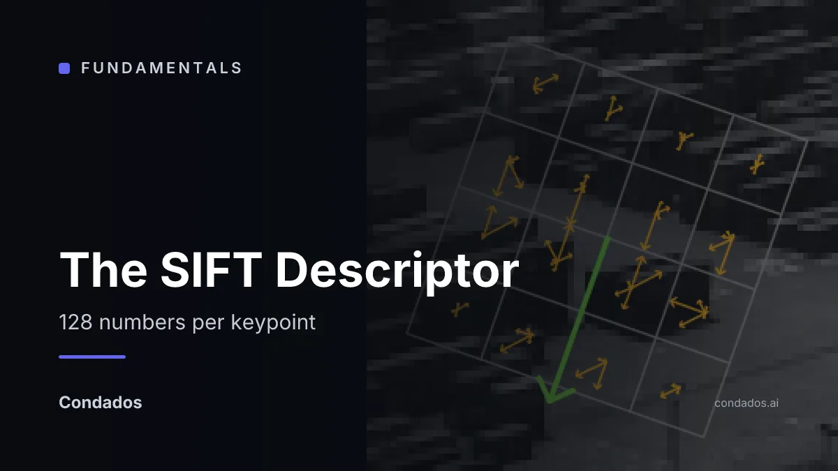
The SIFT descriptor turns the neighbourhood of a keypoint into a list of 128 numbers, built so that the same spot photographed again, turned, closer or under different light, gives nearly the same list. The animation shows why that matters: a copy of the harbour photo turns and shrinks, and the matches keep landing on the same places.
- Blur at many sizes (lesson 2).
- Keep the extrema, 3. refine and test them, and 4. give each a direction (lesson 3): every keypoint now has a position, a size and a direction.
- Describe it: lay a 4×4 grid over its neighbourhood, at its size and turned to its direction, and count the gradient directions in each cell. That is this lesson.
- Match the descriptions between photos (lesson 5).
You have met descriptors like this in:
- Panorama stitching and 3-D reconstruction, which pair points between photos by comparing them (structure from motion).
- Pedestrian detectors of the 2000s, whose HOG feature (histograms of oriented gradients) is the same idea over a whole window.
- Recognising a book cover, a painting or a landmark from a phone photo, which compared such descriptors against a database before learned features.
- Learned descriptors such as XFeat, DISK and ALIKED (unit 3.4, not written yet), which are trained to do this job and are still scored the way this lesson scores SIFT.
Each step of the descriptor exists for one kind of change, and removing it breaks matching under that change. On photo A against a copy of itself turned by 45°, describing every point in the photo’s own axes instead of its own direction takes the correct matches from 1,927 to 0. Against the same photo at half the contrast, skipping the normalization takes them from 907 to 146. The clip at 0.2 barely changes anything on these tests (907 against 907).
Where we are
Lesson 4 of SIFT, step 5 of its pipeline. Lesson 3 left each keypoint with a position, a size and a direction; this lesson uses all three. The 128 numbers it produces are what lesson 5 compares between photos, and the yardstick is still lesson 1’s: a description is good if the same spot gets the same description in the other photo, and a different spot gets a different one.
The obvious description, and where it fails
The most direct way to describe a neighbourhood is to keep its pixels: cut a small square around the keypoint and compare squares between photos by how well their brightness correlates. The hub measures that with 11×11 patches compared by normalized cross-correlation, against SIFT, on the harbour pair:
| second photo | patch: correct matches | SIFT: correct matches |
|---|---|---|
| photo B as taken | 180 of 204 | 420 of 440 |
| photo B turned 20° | 0 of 13 | 433 of 457 |
| photo B at 0.71 of its size | 5 of 34 | 254 of 272 |
The patch works when the second photo is taken from almost the same place, and fails as soon as it turns or zooms: turned by 20°, every pixel of the square has moved to another position, so the square that should match is a different square. Lowe makes the same point: correlation of image patches “is highly sensitive to changes that cause misregistration of samples” [1]. Mikolajczyk and Schmid later compared ten descriptors, cross-correlation among them, under different image transformations, and found that “the SIFT based descriptors perform best” [4].
SIFT changes three things about the patch. It cuts the square at the keypoint’s size, which lesson 2 made available. It turns the square to the keypoint’s direction, from lesson 3. And instead of the pixels themselves it stores their gradients, summarized coarsely enough that a pixel landing one or two positions away still counts in the same place.
Gradient histograms on a 4×4 grid
The gradient at a pixel is the direction in which its brightness rises fastest, and how fast (image gradients). Adding a constant to every pixel leaves it unchanged, which already removes one kind of lighting change.
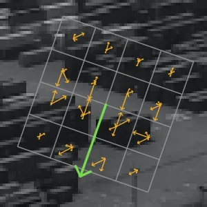
The descriptor lays a square of 4×4 cells over the keypoint, each cell wide, where is the blur at which the keypoint was found. In each cell it adds up the gradients in a histogram of 8 directions, 45° apart, each gradient counting by its strength and by a Gaussian weight that fades with distance from the keypoint [1]:
Each gradient is also shared between the two nearest cells across and down and the two nearest of the 8 directions, Lowe’s trilinear interpolation, so that a gradient moving across a cell or a bin border changes the numbers gradually instead of all at once [1]. Szeliski describes the same layout in §7.1.2 [2].
Turned to the keypoint’s direction
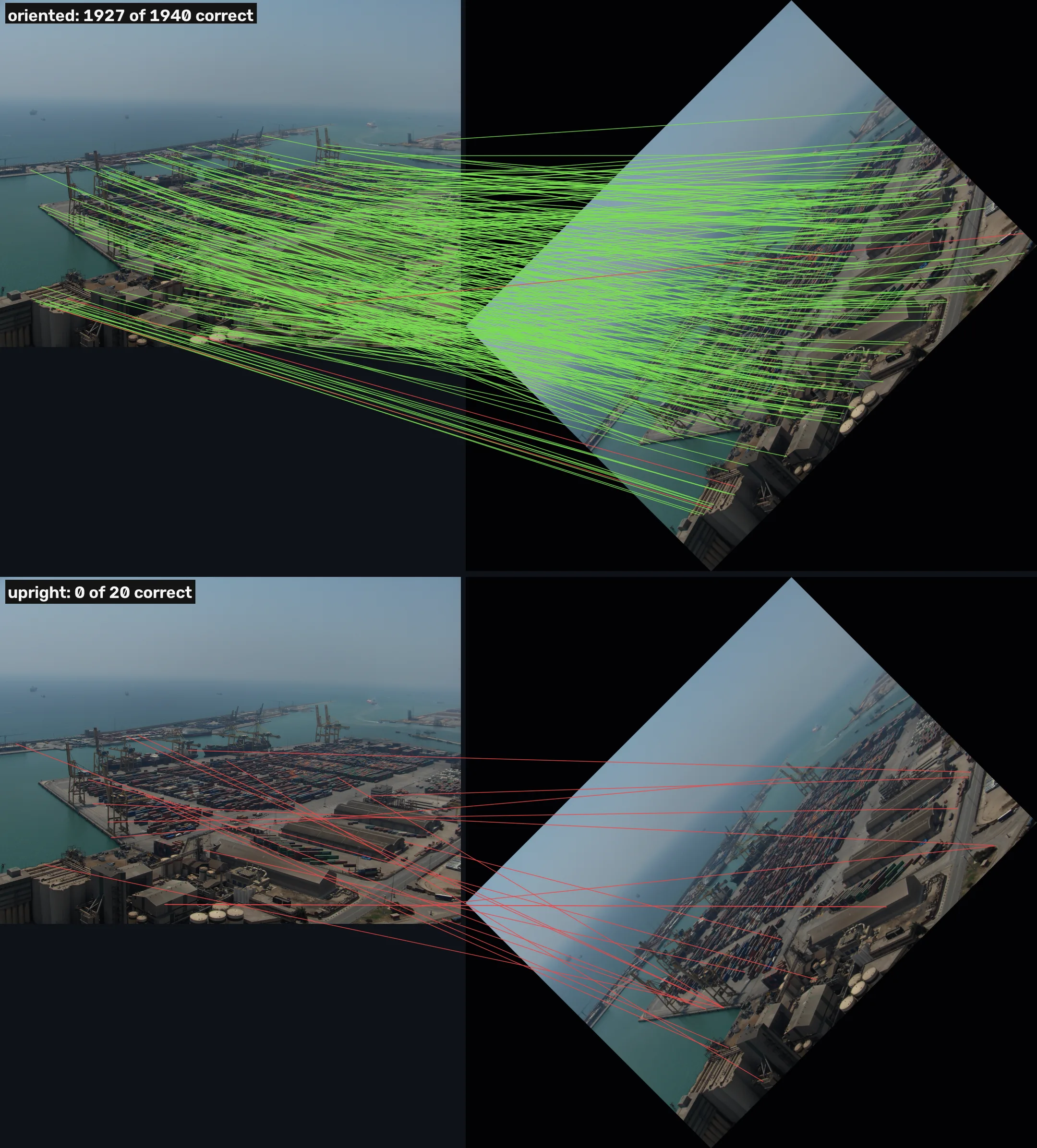
A grid fixed to the photo’s axes describes a turned photo with turned gradients in other cells, so the numbers change. SIFT lays the grid along the keypoint’s direction and measures every gradient direction relative to it [1]. The test: match photo A against copies of itself turned by a known angle, once with each keypoint’s own direction and once with every keypoint forced upright (angle 0), and count matches that land within 3 px of where the point went. The keypoints are those of lesson 3’s from-scratch detector, one per place (2,896 on photo A).
| turned by | own direction: correct | upright: correct |
|---|---|---|
| 0° | 2,896 | 2,896 |
| 10° | 1,867 | 1,536 |
| 20° | 1,921 | 27 |
| 45° | 1,927 | 0 |
What it means: upright descriptors survive a small turn, because each cell’s histogram moves by less than one 45° bin at 10°. At 20° they are gone, and at 45° not one of the 20 matches the ratio test keeps is right. With its own direction, the descriptor matches as many points at 45° as at 10°.
Normalized, then clipped
Brighten or darken a photo by a factor and every gradient is multiplied by the same factor, so every one of the 128 numbers is too. Dividing the vector by its length cancels that: a contrast change becomes no change at all [1]. The test: match photo A against the same photo at half its contrast.
| change | full descriptor | no normalization | no clip |
|---|---|---|---|
| contrast ×0.5 | 907 correct (0.982) | 146 (0.859) | 907 (0.969) |
| gamma 0.5 | 2,016 (0.989) | 1,955 (0.991) | 2,015 (0.990) |
| ×1.8, saturating | 2,609 (0.997) | 46 (0.630) | 2,605 (0.996) |
Correct matches, with the share of kept matches that are correct in brackets. Gamma 0.5 brightens the darks more than the lights; ×1.8 brightens everything and clips about a third of the photo (35% of its pixels) at white. Detection runs on the changed photo too, which is why the counts differ between rows.
Without normalization, a descriptor from the half-contrast photo is half as long as its partner, and is often nearer to some other point’s descriptor: 146 correct matches against 907. Saturation breaks it further, to 46. Gamma changes contrast differently for darks and lights, so normalization does less there, and on this photo the unnormalized descriptor almost keeps up.
Then the clip. After normalizing, any of the 128 values above 0.2 is cut to 0.2 and the vector normalized again. Lowe’s reason: camera saturation and light falling on 3-D surfaces at different angles “can cause a large change in relative magnitudes for some gradients, but are less likely to affect the gradient orientations”, so a single strong gradient should not decide a match; he chose 0.2 by experiment [1]. Every descriptor on photo A has at least one value above 0.2 before the clip, a median of 6.
On these tests the clip does almost nothing: the same 907 correct matches at half contrast, with a slightly lower share of correct ones without it, and 2,015 against 2,016 under gamma. A uniform change of the whole photo is the case normalization already handles; the case Lowe built the clip for, light that changes differently on different surfaces, is not one these warps produce. I did not test it.
This explains the five values of 147 in the worked example: they are the five entries the clip cut to 0.2. Normalizing again scaled the whole vector by the same factor, and , so after the clip the vector’s length was 0.697.
How close is this to OpenCV?
The from-scratch descriptor of the companion repo (features/sift_scratch.py) follows OpenCV’s
calcSIFTDescriptor [3]. On the 3,510 keypoints of photo A, its 128 numbers equal
OpenCV’s byte for byte on 87.15% of them; on the rest they differ by rounding, with a median
cosine of 1.0 and 0.9996 at the 1st percentile.
The cell below is shorter and simplified, to fit on a page: it samples a 16×16 grid of points instead of every pixel of the window, assigns each sample to one cell instead of sharing it between neighbouring cells, and blurs the photo itself instead of reading the pyramid level. It still shares each gradient between the two nearest directions, uses the same Gaussian weight and normalizes and clips the same way. It fetches photo A as the site serves it, a WebP of the same 960×723 photo.
import numpy as np
import cv2

img = cv2.imread("barcelona-a.webp", cv2.IMREAD_GRAYSCALE)
sift = cv2.SIFT_create()
kps = sift.detect(img, None)
# a mid-sized keypoint, so its window is a few dozen pixels wide
kp = max((k for k in kps if 8 < k.size < 12), key=lambda k: k.response)
print(f"keypoint at ({kp.pt[0]:.1f}, {kp.pt[1]:.1f}),",
      f"size {kp.size:.1f} px, angle {kp.angle:.1f}°")

def describe(gray, kp, normalize=True):
    """4x4 cells x 8 directions around kp, rotated by kp.angle."""
    sigma = kp.size / 2               # the keypoint's blur, in pixels
    cell = 3 * sigma                  # one cell of the 4x4 grid
    L = cv2.GaussianBlur(gray.astype(np.float32), (0, 0), sigma)
    gx = cv2.Sobel(L, cv2.CV_32F, 1, 0, ksize=1)
    gy = -cv2.Sobel(L, cv2.CV_32F, 0, 1, ksize=1)  # y up
    t = np.radians(360 - kp.angle)    # the keypoint's direction
    # sample points on a 16 x 16 grid in the keypoint's frame
    u = (np.arange(16) - 7.5) / 4     # in cells, -1.875 .. 1.875
    U, V = np.meshgrid(u, u)
    x = kp.pt[0] + cell * (U * np.cos(t) + V * np.sin(t))
    y = kp.pt[1] + cell * (U * np.sin(-t) + V * np.cos(t))
    sx = cv2.remap(gx, x.astype(np.float32), y.astype(np.float32),
                   cv2.INTER_LINEAR)
    sy = cv2.remap(gy, x.astype(np.float32), y.astype(np.float32),
                   cv2.INTER_LINEAR)
    mag = np.hypot(sx, sy) * np.exp(-(U**2 + V**2) / 8)
    ang = (np.degrees(np.arctan2(sy, sx)) - np.degrees(t)) % 360
    hist = np.zeros((4, 4, 8))
    o = ang / 45                      # bins centred on 0, 45, 90, ...
    b0 = np.floor(o).astype(int)
    w1 = o - b0                       # split between the two nearest
    for i in range(16):
        for j in range(16):
            hist[i // 4, j // 4, b0[i, j] % 8] += mag[i, j] * (1 - w1[i, j])
            hist[i // 4, j // 4, (b0[i, j] + 1) % 8] += mag[i, j] * w1[i, j]
    v = hist.ravel()
    if not normalize:
        return v
    v = v / np.linalg.norm(v)
    v = np.minimum(v, 0.2)            # no single gradient dominates
    v = v / np.linalg.norm(v)
    return np.clip(np.round(v * 512), 0, 255)

mine = describe(img, kp)
_, theirs = sift.compute(img, [kp])
theirs = theirs[0]
cos = mine @ theirs / np.linalg.norm(mine) / np.linalg.norm(theirs)
print("numbers:", mine.size, " cosine with OpenCV's:", round(cos, 3))
print("largest difference:", int(np.abs(mine - theirs).max()), "of 255")
print("ours  [:8]", mine[:8].astype(int))
print("OpenCV[:8]", theirs[:8].astype(int))keypoint at (406.7, 707.1), size 11.7 px, angle 75.1° numbers: 128 cosine with OpenCV's: 0.958 largest difference: 55 of 255 ours [:8] [35 14 6 6 0 2 1 5] OpenCV[:8] [46 26 4 7 3 4 4 17]
A cosine of 1 means the two vectors point the same way. Here it is 0.958, with the largest of the 128 numbers 55 apart: the price of the three simplifications, which the full version in the companion repo does not pay.
The upright test of the table above, on 500 points per photo so that it runs in the page:
# Photo A against a copy of itself turned by 45 degrees.
def turned(gray, deg):
    h, w = gray.shape
    M = cv2.getRotationMatrix2D((w / 2, h / 2), deg, 1.0)
    c, s = abs(M[0, 0]), abs(M[0, 1])
    W, H = int(h * s + w * c), int(h * c + w * s)
    M[0, 2] += W / 2 - w / 2
    M[1, 2] += H / 2 - h / 2
    return cv2.warpAffine(gray, M, (W, H)), M

def points(gray, n=500):
    """The n strongest keypoints, one per place (no orientation copies)."""
    seen, out = set(), []
    for k in sorted(sift.detect(gray, None), key=lambda k: -k.response):
        key = (round(k.pt[0], 1), round(k.pt[1], 1))
        if key not in seen:
            seen.add(key)
            out.append(k)
    return out[:n]

def correct_matches(deg, upright):
    img2, M = turned(img, deg)
    ka, kb = points(img), points(img2)
    if upright:                      # throw the direction away
        for k in ka + kb:
            k.angle = 0.0
    ka, da = sift.compute(img, ka)
    kb, db = sift.compute(img2, kb)
    good = [m for m, n in cv2.BFMatcher().knnMatch(da, db, k=2)
            if m.distance < 0.75 * n.distance]
    p = np.array([ka[m.queryIdx].pt for m in good]).reshape(-1, 2)
    q = np.array([kb[m.trainIdx].pt for m in good]).reshape(-1, 2)
    where = p @ M[:, :2].T + M[:, 2]   # where each point went
    ok = np.linalg.norm(where - q, axis=1) <= 3
    return int(ok.sum()), len(good)

for deg in (45,):
    print(f"{deg}°  oriented: %d of %d correct" % correct_matches(deg, False))
print(f"{deg}° upright: %d of %d correct" % correct_matches(deg, True))45° oriented: 290 of 299 correct 45° upright: 0 of 8 correct
The orientation copies of lesson 3 are left out on purpose: forced upright, two copies of the same point would have identical descriptors, and the ratio test of lesson 5 would reject both as ambiguous.
In the wild
The orientation test on templeR0001, a 640×480 photo of a plaster temple from the Middlebury multi-view dataset [6], against a copy turned by 45°: with each keypoint’s own direction, 487 of 496 matches are correct (0.982); upright, 0 of 13.
What it means: the same collapse as on the harbour, on a plaster object against a black background. Without a direction, a turn of 45° leaves nothing to match on either photo.
Where this breaks
A change of viewpoint is outside what it was built for. Turning, zooming and uniform lighting changes are handled step by step. A change of viewpoint around a 3-D object moves pixels in ways no turn or zoom describes, and lesson 5 measures how quickly matching falls off when the camera walks around the temple.
It needs a direction it can trust. Every number is measured relative to the keypoint’s direction, so a wrong direction from lesson 3 gives a wrong description. That is why SIFT makes a copy of a point whose second direction is close to its first.
A mirror image is a different descriptor. Flipping the photo left to right reverses the order of the directions in every cell, and no turn undoes that.
Repeated texture gives repeated descriptors. Windows of the same building, containers of the same size: their neighbourhoods look alike, so their 128 numbers do too. The descriptor cannot tell them apart; lesson 5’s ratio test is how SIFT notices.
On these tests the clip changed little. On every change tested, removing it moved the correct matches by at most four. Its case is uneven lighting on 3-D surfaces, which these tests do not contain.
What this means for your pipeline
- Photos turned by more than about 10° need oriented descriptors: upright ones fell from 1,536 correct at 10° to 27 at 20° and 0 at 45°, while oriented ones held at about 1,900.
- Keep the normalization: without it, half the contrast took correct matches from 907 to 146.
- Do not count on the clip on your data without testing it: on these changes it moved the correct matches by at most four.
- A raw patch is a fair choice only when the two photos are nearly aligned: turned 20°, patches gave 0 correct matches and SIFT 433.
Exercises
- Normalize and clip. Write
normalize(v): divide by the length, cut every value above 0.2 to 0.2, divide by the new length. The check tries it on a vector with one large entry, and on the same vector doubled.
import numpy as np

def normalize(v):
    return v  # unit length, clip at 0.2, unit length again

v = np.r_[10.0, np.ones(127)]
print(normalize(v)[:3])
print(normalize(2 * v)[:3])- Predict, then run. In the cell “Own direction against upright”, change
(45,)to(10,). Will the upright descriptors keep most of their matches, or lose them as at 45°? - Break it. Describe the same keypoint on the photo and on the photo at half contrast, without normalizing, and compare the distance between the two descriptors with their length. Then normalize. Add this after the first cell:
dark = (img * 0.5).astype(np.uint8)
for norm in (False, True):
    a, b = describe(img, kp, norm), describe(dark, kp, norm)
    print("normalize", norm,
          "distance:", round(float(np.linalg.norm(a - b)), 1),
          "length:", round(float(np.linalg.norm(a)), 1))
What you should see
Answer 1 is the solution cell in section 5 of the unit notebook, sift.ipynb. Answers 2 and 3
come from running the modified cells on this page (OpenCV 4.11) and the same modified cells on
OpenCV 5.0; where the two differ, both are given.
[0.2583 0.0857 0.0857]for both lines. The large entry was 0.664 of the unit vector before the clip; the clip cuts it to 0.2 and the second normalization lifts everything back to unit length. Doubling the vector changes nothing.- Most of them: at 10°, 265 of 268 upright matches are correct against 300 of 308 with each keypoint’s own direction (266 of 270 and 298 of 306 on 5.0). A 10° turn moves each histogram by less than one 45° bin.
- Without normalization the distance is 128.4 for a vector 256.6 long: half its length, because the half-contrast descriptor is half the size. Normalized, the distance falls to 2.4 (2.0 on 5.0) on a vector 512.8 long.
Check yourself
Four questions on this lesson. Pick an answer to see why it is right or wrong.
Where do the 128 numbers of a SIFT descriptor come from?
4 × 4 × 8 = 128. Each cell sums gradient strength in 8 directions, 45 degrees apart.
Photo A against a copy turned 45 degrees. What happens to the correct matches if every descriptor is computed upright, ignoring the keypoint direction?
A fixed grid sees the turned gradients in other cells and other bins. Upright descriptors survive 10 degrees (1,536 correct) and are gone by 20 (27).
Which change of the photo does normalizing the 128 numbers to unit length cancel?
At half contrast, skipping normalization takes the correct matches from 907 to 146. Adding a constant is already removed by the gradient.
What did removing the clip at 0.2 do on this lesson’s tests?
Lowe added the clip for light that changes differently on different 3-D surfaces, which uniform changes of the whole photo do not produce.
Next
Lesson 5: matching and Lowe’s ratio test compares these 128 numbers between the two harbour photos and decides which pairs to trust. The yardstick stays lesson 1’s, and the keypoints come from lesson 3.
Run it: every code block on this page has a cell in the unit’s notebook, open it in Colab.
Further reading
- The source: Lowe 2004 [1], §6 and §6.1, for the descriptor in two pages, including why gradients that may shift a few samples still land in the same histogram, and where 0.2 came from.
- The book: Szeliski §7.1.2 [2], for SIFT next to the descriptors that followed it (PCA-SIFT, RootSIFT, GLOH), with the same 4×4×8 layout drawn out.
- The comparison: Mikolajczyk and Schmid’s evaluation [4], for SIFT against other local descriptors under rotation, zoom, blur and light.
- Related on CondadosAI: Image gradients is what every cell counts; learned local features, the descriptors trained to replace this one, are unit 3.4 (not written yet).
References
[1] Lowe, D. G. (2004). Distinctive Image Features from Scale-Invariant Keypoints. International Journal of Computer Vision, 60(2), 91–110: §6 “The local image descriptor” (correlation of patches “highly sensitive to changes that cause misregistration of samples”) and §6.1 “Descriptor representation” (4×4 histograms of 8 directions, trilinear interpolation, normalization, the 0.2 threshold “determined experimentally using images containing differing illuminations for the same 3D objects”). Section titles read off the author’s accepted manuscript. doi:10.1023/B:VISI.0000029664.99615.94
[2] Szeliski, R. (2022). Computer Vision: Algorithms and Applications (2nd ed.), §7.1.2 “Feature descriptors”, p. 434; SIFT on pp. 435–436 (page numbers of the final draft, Sept. 2021). Springer. Free PDF
[3] OpenCV 4.11.0 source, modules/features2d/src/sift.simd.hpp: calcSIFTDescriptor (the 4×4×8 histogram, the clip at SIFT_DESCR_MAG_THR = 0.2 and the scaling by SIFT_INT_DESCR_FCTR = 512). calcSIFTDescriptor at line 709, the clip at lines 914 and 943, the constants at lines 84–117. Commit 31b0eee.
[4] Mikolajczyk, K., & Schmid, C. (2005). A Performance Evaluation of Local Descriptors. IEEE Transactions on Pattern Analysis and Machine Intelligence, 27(10), 1615–1630. doi:10.1109/TPAMI.2005.188
[5] Pap3rinik. BarcelonaHarbour1.jpg and BarcelonaHarbour2.jpg. Wikimedia Commons, public domain. commons.wikimedia.org

[6] Seitz, S. M., Curless, B., Diebel, J., Scharstein, D., & Szeliski, R. (2006). A Comparison and Evaluation of Multi-View Stereo Reconstruction Algorithms. CVPR 2006, pp. 519–528. doi:10.1109/CVPR.2006.19. The Middlebury multi-view datasets: vision.middlebury.edu/mview