
Before this unit: Edge detection
Probabilistic Hough Transform: Lane Segments with OpenCV's HoughLinesP
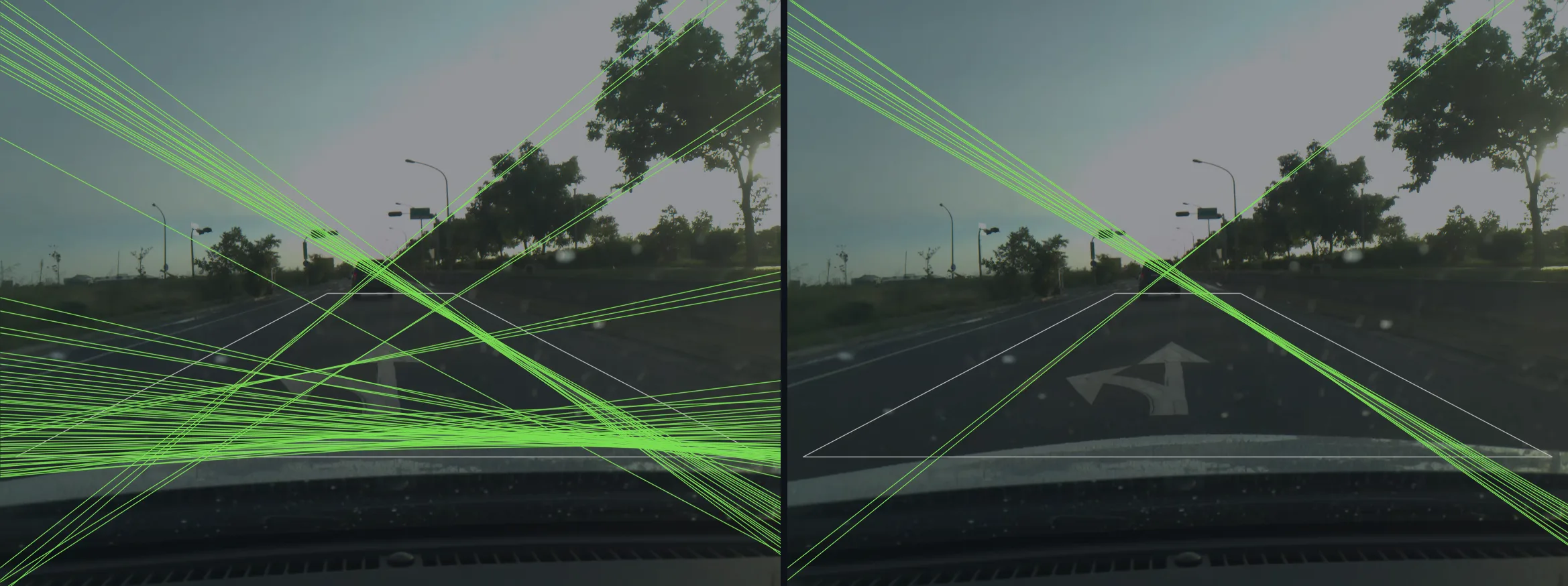
The full Hough vote reports lines that are not lanes. On a hard dashcam frame it gives 72 lines, 18 of them on paint; dropping near-horizontal lines and voting within ±5° of each pixel's gradient leaves 13, all on paint. Over 299 frames that takes the median share of lines on paint from 50% to 100%, and leaves 108 frames with no line at all.
The probabilistic Hough transform finds straight segments, each with two ends, by letting a random sample of edge pixels vote and following each line it detects along the image. Below, a lane-keeping display built on the segments it returns, on seven seconds of freeway.

cv2.HoughLinesP segments: each stops where its lane marking stops, and a dashed line is joined across its gaps. The segments on each side of the car are fitted with one line, averaged over the last few frames and extended up the road; the lane between the two lines is filled. Video: comma2k19 (comma.ai, MIT).You have met it in:
- Lane-detection tutorials, almost all of which call
cv2.HoughLinesPon a Canny map. - Document scanners, which need the four sides of a page as segments so they can intersect them into corners.
- Court and pitch line detection in sports graphics.
- Robots and drones that follow corridor walls, floor tape or power lines.
Most of the lines the plain vote reports on a real road are not lanes, and three changes clean that up: vote only in the direction each edge faces, ignore lines no lane can follow, and return segments with ends instead of endless lines. Over 299 dashcam frames the first two take the median share of lines on paint from 50% to 100%, at a cost: the frames where no line survives rise from 42 to 108.
Where we are
Lesson 2 of Boundary detection. Lesson 1 built the global vote [4] and found its problems: one lane line becomes a fan of lines, the threshold and bin size move the answer, and on a typical frame half the lines are guard rails, cars and shadows. All of it comes from every pixel voting at every angle, although image gradients already told us which way each edge runs, and although a lane seen from a car is never flat.
Fix 1: restrict the vote
At an edge pixel the gradient points across the edge, which is the direction of the line’s normal, so the gradient’s angle is already an estimate of . Szeliski calls voting for that single cell the better approach whenever the gradient is reliable, and suggests a hybrid where each pixel votes for a few angles around its estimate [1]. That hybrid is what this lesson measures: each pixel votes for the angles within degrees of its gradient direction, instead of all 180.
The second restriction is about lanes, not about images: from a car, a lane line is never within 20° of horizontal. Lines with between 70° and 110° are dropped. A horizon, a bumper, the hood’s edge and the shadow of a bridge all live there.
On the clean frame of lesson 1 the restrictions change little: its 15 lines were already all on paint. On a harder frame of the same dataset they change everything:
| frame 2904 of the sample | lines over 60 | on paint | paint covered |
|---|---|---|---|
| full vote | 72 | 18 | 100% |
| ±5° and no near-horizontal lines | 13 | 13 | 100% |
Over all 299 frames:
| vote | lines (median) | on paint (median share) | paint covered (median) | frames with no line |
|---|---|---|---|---|
| full | 17 | 50% | 75.7% | 42 |
| no near-horizontal lines | 8 | 100% | 63.7% | 92 |
| ±5° and no near-horizontal lines | 3 | 100% | 45.4% | 108 |
Each restriction raises precision and lowers how often anything is found. The darker frames of the dataset are where the line count falls to zero, which is the honest limit of a method that starts from Canny on a dim road.
Now you try
The clean frame, voting along the gradient. Narrow from 5 to 2 and watch the lines over the threshold fall from 12 to 9, as pixels whose gradient strays stop voting for their line. The near-horizontal toggle changes nothing on this frame, which has no flat line over the threshold; frame 2904 above is where it matters.
Fix 2: segments with ends
A cell is an infinite line across the whole frame. A lane marking is a segment, and a dashed one is a row of segments; the ends are what the next step needs.
The progressive probabilistic Hough transform of Matas, Galambos and Kittler [2] changes the voting order. Edge pixels are drawn one at a time in random order and vote. After each vote it asks whether any cell has more votes than chance would give. When one does, it walks along that line in the image, collects the pixels that support it into a segment, takes their votes back out of the accumulator and removes them from the pixels still to be drawn. A long line is found after a small fraction of its pixels have voted, and most pixels never vote. The authors note it combines with gradient restriction without conflict. A segment’s direction is still read off a 1 px by 1° cell; lesson 3 fits a line to the pixels themselves.
cv2.HoughLinesP is that algorithm with three settings: a vote threshold, the shortest segment
to return (minLineLength) and the longest gap to bridge within one segment (maxLineGap)
[3]. The gap is what joins a dashed lane line into one segment.
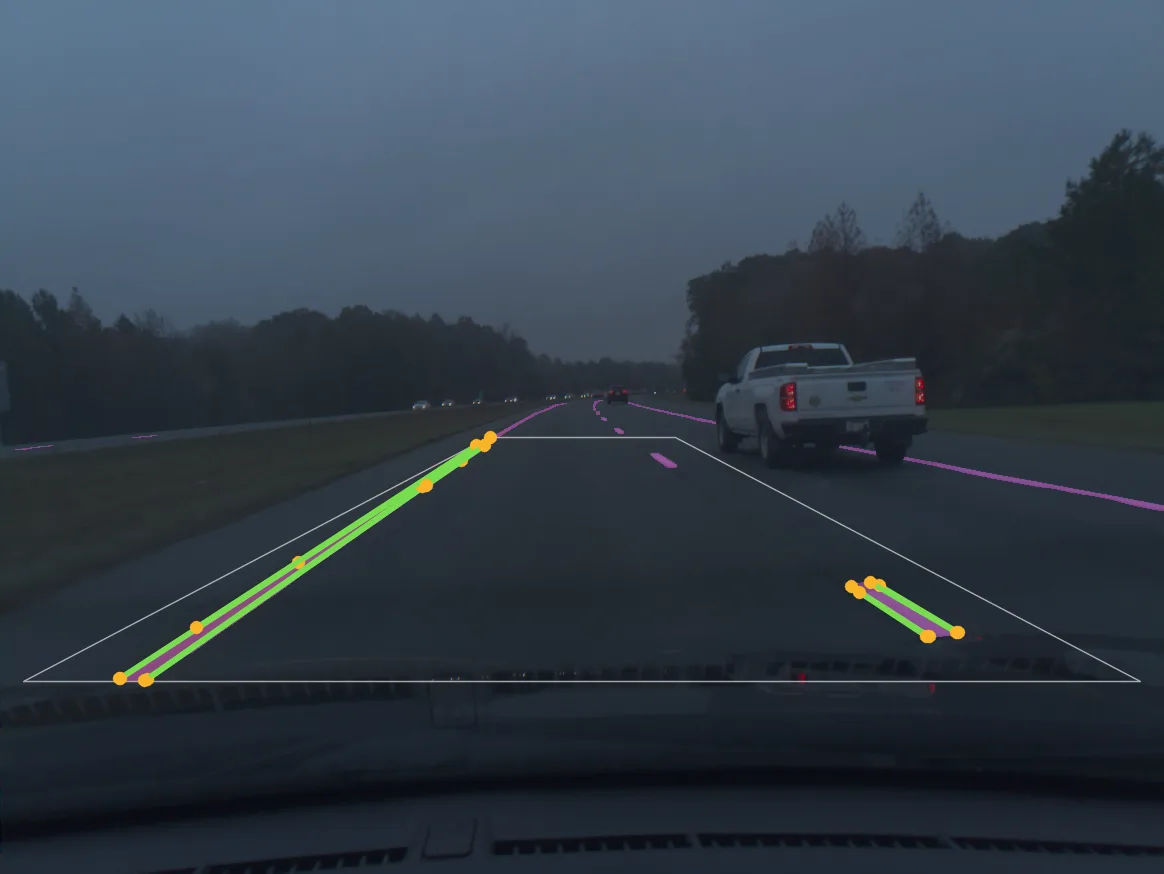
HoughLinesP(threshold 40, minLineLength 40, maxLineGap 20) on the clean frame: 10
segments, all on paint, covering 79.8% of it. comma10k (comma.ai, MIT).How close is this to OpenCV?
OpenCV has no gradient-restricted HoughLines, so the check runs the other way: the restricted
accumulator in NumPy, against the set of lines OpenCV’s full accumulator returns on the frame
(comma10k, MIT [5]). Then HoughLinesP, run twice. The edge map is unit 3.1’s
Canny inside the road trapezoid, as in every lesson.
import numpy as np
import cv2

img = cv2.imread("highway.webp")
h, w = img.shape[:2]
blur = cv2.GaussianBlur(
    cv2.cvtColor(img, cv2.COLOR_BGR2GRAY), (0, 0), 1.4)
road = np.zeros((h, w), np.uint8)
corners = [(0.02, 0.78), (0.42, 0.50),
           (0.58, 0.50), (0.98, 0.78)]
cv2.fillPoly(road, [np.array(
    [(fx * w, fy * h) for fx, fy in corners], np.int32)], 255)
edges = cv2.Canny(blur, 25, 75) & road

gx = cv2.Sobel(blur, cv2.CV_32F, 1, 0)
gy = cv2.Sobel(blur, cv2.CV_32F, 0, 1)
ys, xs = np.nonzero(edges)
grad = np.degrees(np.arctan2(gy, gx)) % 180
centre = np.rint(grad[ys, xs]).astype(int)

# lesson 1's angle table, built the way OpenCV builds it
cos_t = np.zeros(180, np.float32)
sin_t = np.zeros(180, np.float32)
ang = np.float32(0)
for t in range(180):
    cos_t[t] = np.cos(np.float64(ang))
    sin_t[t] = np.sin(np.float64(ang))
    ang = np.float32(ang + np.float32(np.pi / 180))

n_rho = 2 * (w + h) + 1
half = (n_rho - 1) // 2
acc = np.zeros((n_rho, 180), np.int32)
k = 5
x32, y32 = xs.astype(np.float32), ys.astype(np.float32)
for off in range(-k, k + 1):
    t = (centre + off) % 180
    r = np.rint(x32 * cos_t[t] + y32 * sin_t[t])
    np.add.at(acc, (r.astype(int) + half, t), 1)

print("votes cast:", len(xs) * (2 * k + 1))votes cast: 19239
A = np.pad(acc, 1)
m = A[1:-1, 1:-1]
peak = ((m > 60) & (m > A[:-2, 1:-1])
        & (m >= A[2:, 1:-1]) & (m > A[1:-1, :-2])
        & (m >= A[1:-1, 2:]))
# the lane prior: nothing within 20 degrees of flat
ours = [(r, t) for r, t in zip(*np.nonzero(peak))
        if not 70 <= t <= 110]
ref = cv2.HoughLines(edges, 1, np.pi / 180, 60)
cv = {(round(rr) + half, round(np.degrees(tt)))
      for rr, tt in ref.reshape(-1, 2)}
print("restricted lines:", len(ours),
      " also in OpenCV's full set:",
      sum((r, t) in cv for r, t in ours), "of", len(cv))

seg1 = cv2.HoughLinesP(edges, 1, np.pi / 180, 40,
                       minLineLength=40, maxLineGap=20)
seg2 = cv2.HoughLinesP(edges, 1, np.pi / 180, 40,
                       minLineLength=40, maxLineGap=20)
print("segments:", len(seg1),
" same on a second run:", np.array_equal(seg1, seg2))restricted lines: 12 also in OpenCV's full set: 12 of 15 segments: 10 same on a second run: True
All 12 restricted lines are lines OpenCV’s full accumulator also reports, so the restriction
finds no new lines on this frame; it keeps 12 of the 15. HoughLinesP returns the same 10
segments on every run because OpenCV seeds its random sampler with a fixed value
[3]: random in the statistical sense, reproducible in the engineering sense, which is
the useful combination for a test suite.
In the wild
A photograph of a sheet of paper lying at an angle on a bench, as a document scanner would see
it, with the same HoughLinesP at its own settings (threshold 90, shortest segment 80, gap 5):
| edge pixels | 10,325 |
| full-vote lines over 90 votes | 36 |
HoughLinesP segments | 10 |
| the four longest | 283, 262, 258 and 185 px |
| their directions | 52.0°, 52.0°, 52.9° and 142.0° |
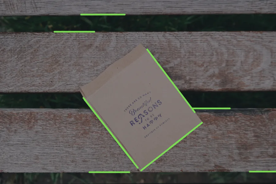
What it means: the three longest segments are the page’s long sides and agree on its tilt to within a degree; the fourth is a short side at 90° from them, as a page’s should be. That is what a scanner needs to straighten the page with a homography.
Where this breaks
Two more thresholds, no principled values. On the clean frame, at a vote threshold of 40:
minLineLength \ maxLineGap | 5 | 20 | 60 |
|---|---|---|---|
| 20 | 18 (79.4%) | 11 (84.0%) | 11 (87.6%) |
| 40 | 17 (73.1%) | 10 (79.8%) | 11 (87.6%) |
| 80 | 9 (59.6%) | 8 (70.0%) | 9 (81.1%) |
Segments, with the share of the paint they cover in brackets. Every segment in the table is on paint on this frame. A longer gap joins the dashes and covers more paint; on a frame with a guard rail beside the lane, the same gap is free to join the two.
Precision on typical frames is still low. Over 299 frames, HoughLinesP with these settings
returns a median of 15 segments on the brighter frames and 10.5 on the darker ones, of which a
median 30% and 47% lie on paint. The segment stage here has no lane prior; I did not measure it
with one.
Fewer false lines means more frames with none. The restrictions that took precision to 100% also took the frames with no line from 42 to 108 of 299. A lane-keeping system needs an answer on every frame; this method gives a clean one or none, and the “none” is common at night.
A line is still only a line. A lane on a bend is a curve, and so is the rim of a wheel.
Exercises
- Which angles does one pixel vote for? Write
votes(direction, k), returning the whole-degree values in that a pixel with gradient directiondirectionvotes for. Mind the wrap: a pixel at 178° with votes for 175 to 179 and 0 and 1.
def votes(direction, k):
    return []  # whole-degree thetas in [0, 180)

print(sorted(votes(178.2, 3)))
print(sorted(votes(61.39, 5)))- Predict, then run. Set
k = 2in the first cell and rerun both. How many lines clear 60 votes, and how many votes has the strongest? - Bridge the dashes. Run
cv2.HoughLinesPwithmaxLineGap5, 20 and 60 atminLineLength=40and count the segments. Before running, guess which gap gives the fewest.
What you should see
These come from section 2 of the unit notebook, boundary_detection.ipynb, and are the same on
OpenCV 4.11 (this page) and 5.0.
[0, 1, 175, 176, 177, 178, 179]and 56 to 66.- 9 lines, all on paint, the strongest with 302 votes.
- 17, 10 and 11. The gap of 20 joins the dashes into fewer, longer segments; at 60 the count is one higher and the paint covered rises from 79.8% to 87.6%.
Check yourself
Four questions on this lesson. Pick an answer to see why it is right or wrong.
Why can a pixel vote for only a few angles instead of all 180?
The gradient direction is an estimate of θ. Voting within ±5° of it costs 11 votes per pixel instead of 180, 6.1% of the work.
The lowest of the three worked-example pixels has a gradient at 40.82°, while its line is at 57°. What happens with ±5° voting?
Any pixel whose gradient strays more than k from the line’s normal is lost to that line. The strongest cell drops from 362 votes to 349.
Over 299 frames, the lane prior plus ±5° voting takes the median share of lines on paint from 50% to 100%. What is the cost?
Each restriction raises precision and lowers how often anything is found. The method gives a clean answer or none, and none is common on dark frames.
Which HoughLinesP setting joins the dashes of one lane line into one segment?
maxLineGap is the longest gap bridged within one segment. At 60 px the segments cover 87.6% of the paint against 79.8% at 20, and the same gap can also join a lane to a guard rail beside it.
Next
The vote now returns several short segments per lane marking, each with a direction read off a 1° cell. A car steers by one line per side with a precise angle. Lesson 3 fits that line to the segments, and shows why the fit from school algebra gives a different answer depending on which axis it treats as the error.
References
[1] Szeliski, R. (2022). Computer Vision: Algorithms and Applications (2nd ed.), §7.4.2 “Hough transforms”, pp. 477–479 (Figure 7.47, the oriented Hough transform). Springer. Free PDF
[2] Matas, J., Galambos, C., & Kittler, J. (1998). Progressive Probabilistic Hough Transform. Proceedings of the British Machine Vision Conference 1998. doi:10.5244/C.12.26
[3] OpenCV 4.11.0 source, modules/imgproc/src/hough.cpp, HoughLinesProbabilistic (line 490; the sampler is seeded at line 497), commit 1d3b34d.
[4] Gonzalez, R. C., & Woods, R. E. (2018). Digital Image Processing (4th ed.), ch. 10, §10.2 “Point, Line, and Edge Detection”, Global Processing Using the Hough Transform, p. 799. Pearson.
[5] comma.ai (2020). comma10k: 10k crowdsourced images for training segnets. MIT licence. github.com/commaai/comma10k