Before this unit: Homogeneous coordinates

Rotate, Scale, Shear: Images as 2×2 Matrices

Lesson 1 of Image Alignment. A 2×2 matrix is where it sends the two axes; its determinant is how much it scales area and its SVD is rotate, stretch, rotate. The one thing it cannot do is make parallel lines meet. On a pickleball court, the sidelines are 20.35° apart in the photograph, so the best 2×2 misses every corner by 60 px.

Luis Condados · September 27, 2026

computer-vision geometry homography fundamentals

The court as the camera saw it (green), and the best any 2×2 matrix can do with it (red): a parallelogram, because a linear map keeps parallel lines parallel.

Rotating, zooming or slanting a picture moves every pixel by the same small recipe: two numbers say where one step to the right ends up, two say where one step up ends up. Those four numbers are a 2×2 matrix, and they are all a rotation, a zoom or a slant ever is.

A pickleball court diagram rotating, growing and slanting as the four numbers of its matrix change, with the sidelines staying parallel throughout — The court diagram through a rotation, a zoom and a shear. The four numbers and the determinant are printed underneath; the two green sidelines stay parallel whatever the numbers do.

Where 2×2 transforms do the work:

Photo editors. Rotate, resize and skew are each one 2×2 matrix applied to every pixel [1].
Training data. The random rotations, zooms and shears used to augment images for a neural network are 2×2 matrices chosen at random.
Slanted text. A synthetic italic is a shear: every row moves sideways in proportion to its height.
Scanned pages. A page that went into the scanner slightly rotated is straightened by the inverse rotation.

What a 2×2 cannot do is the reason the rest of this unit exists, and a photograph of a court shows it.

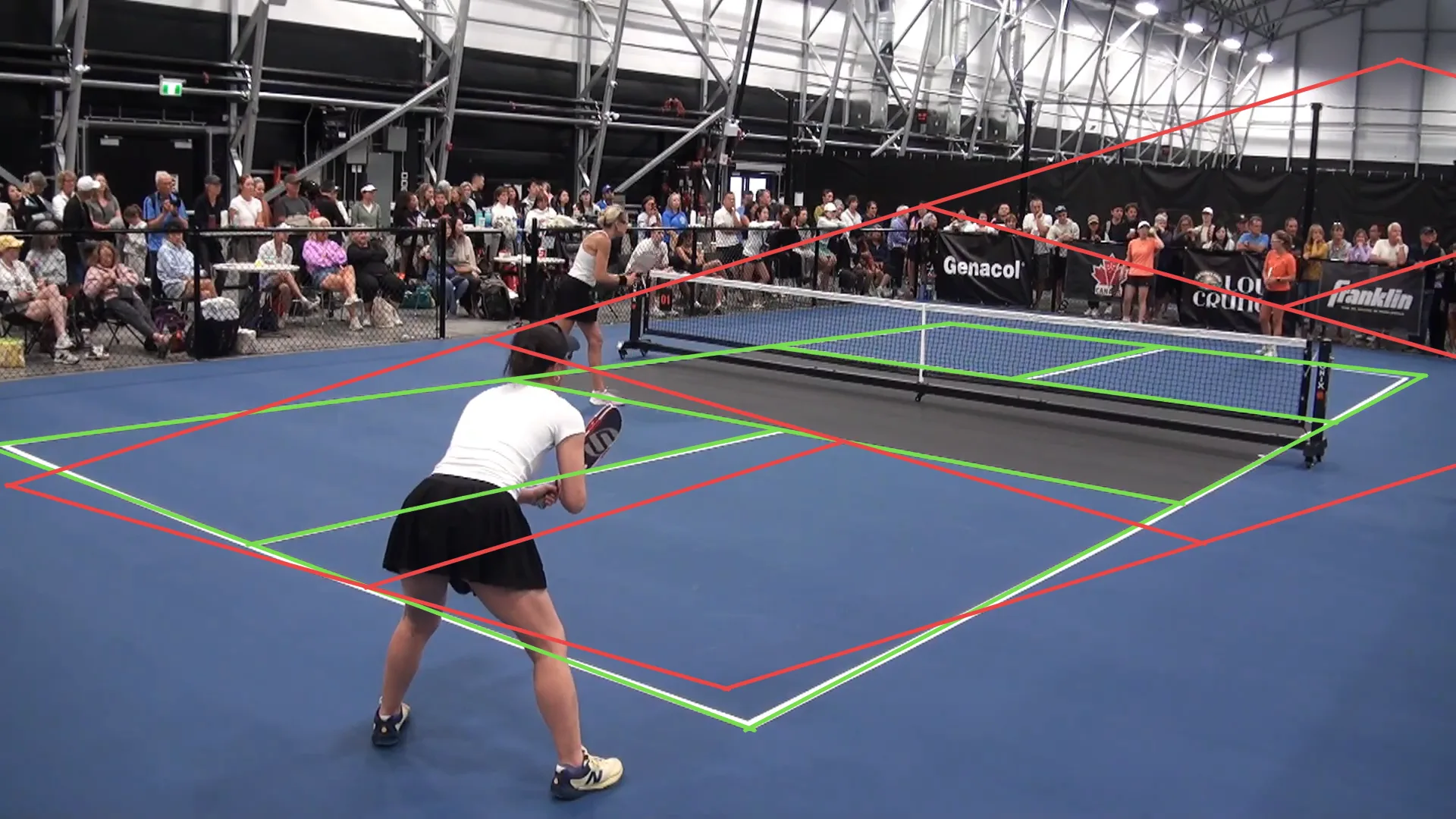
A 2×2 matrix is fully described by two arrows: where it sends one metre along the court and one metre across it. Everything else follows. Its determinant says how much it scales area, and its singular value decomposition says it is always a rotation, a stretch along two axes and another rotation. What it can never do is make two parallel lines meet, and in the photograph of this court the two sidelines are 20.35° apart. The best 2×2 anyone can fit misses every corner by 60.4 px.

Where we are

Part of image alignment. The unit measures everything on one frame of a pickleball final, and the question is how to map the court, in metres, onto the photograph, in pixels. The homogeneous coordinates lesson found the court’s lines and corners in the image. This lesson tries the simplest possible map between the two and finds out why it is not enough.

Two arrows decide everything

Multiply a point $(x, y)$ by a matrix and you get a new point:

\begin{pmatrix} x' \\ y' \end{pmatrix} = \begin{pmatrix} a & b \\ c & d \end{pmatrix}\begin{pmatrix} x \\ y \end{pmatrix} = x\begin{pmatrix} a \\ c \end{pmatrix} + y\begin{pmatrix} b \\ d \end{pmatrix}

The right-hand side is the whole idea. The first column is where the point $(1, 0)$ lands and the second is where $(0, 1)$ lands; every other point is a mix of the two. Rotation, uniform scale, stretching one axis and shearing are all special choices of those two columns [1], and Gonzalez and Woods list the same family as the basic geometric transformations of an image [2].

Two numbers read off any 2×2 tell you what it does.

The determinant $ad - bc$ is the area of the parallelogram the two columns span. A unit square goes in; a parallelogram of area $|ad - bc|$ comes out. Negative means the map mirrors, zero means it squashes the plane onto a line.

The singular value decomposition writes any 2×2 as $M = R_2\,\Sigma\,R_1$ : rotate, stretch by $\sigma_1$ along one axis and $\sigma_2$ along the other, rotate again. No 2×2 does anything that is not those three steps.

Every 2×2 is these three steps. The square’s sides end up with new lengths and new directions, but opposite sides stay parallel at every stage, which is the limit this lesson ends on.

The one thing a 2×2 cannot do

Take a line through $p$ with direction $d$ : the points $p + t\,d$ . Its image is $M p + t\,M d$ , a line with direction $M d$ . A second line with the same direction $d$ maps to a line with the same direction $M d$ . Parallel lines stay parallel under any 2×2, whatever its four numbers are.

The two sidelines of a court are parallel. In frame 45000 they are 20.35° apart, and the previous lesson found where they meet. So no 2×2 can be the map from the court to this photograph. The only question left is how wrong the best one is.

Worked example · The best 2×2 for the near half of the court

Take the four near-half corners in metres and in pixels, subtract each set’s centroid so that translation is out of the way, and solve for the 2×2 that fits best in the least-squares sense:

M = \begin{pmatrix} 137.29 & 156.33 \\ -41.97 & 44.27 \end{pmatrix}\ \text{px per metre}

The columns. One metre along the court (away from the camera) becomes the arrow $(137.3, -42.0)$ px: right and up the frame. One metre across becomes $(156.3, 44.3)$ px: right and slightly down.

The determinant.

\det M = (137.29)(44.27) - (156.33)(-41.97) = 6{,}077.8 + 6{,}561.2 = 12{,}639\ \text{px}^2\ \text{per m}^2

So one square metre of court covers 12,639 pixels, a patch about 112 px on a side.

The SVD. $\sigma_1 = 208.1$ and $\sigma_2 = 60.7$ px per metre, with rotations of −130.8° before the stretch and −178.3° after. The map stretches one direction 3.4 times more than the other, which is what foreshortening looks like when it is forced to be the same everywhere.

What it means: the fit leaves 60.4 px of error at every one of the four corners. And the determinant exposes why. The true area scale, measured from the homography the unit ends up with, is 62,697 px² per m² at the near-right corner and 10,479 at the near-right kitchen corner, six times less, 4.6 m further away. A 2×2 has one determinant for the whole plane, so it has to pick something in between and be wrong at both ends.

import numpy as np

court = np.array([[0.0254, 0.0254], [0.0254, 6.0746], [4.6004, 0.0254], [4.6004, 6.0746]])  # m
image = np.array([[-18.52, 587.39], [987.25, 959.91], [669.68, 500.09], [1555.24, 663.22]])  # px

c0, i0 = court - court.mean(0), image - image.mean(0)
M = np.linalg.lstsq(c0, i0, rcond=None)[0].T        # image ≈ M @ court, both centred
U, s, Vt = np.linalg.svd(M)
print(M.round(2), np.linalg.det(M).round(0), s.round(1))
print(np.linalg.norm(c0 @ M.T - i0, axis=1).round(1))  # [60.4 60.4 60.4 60.4]

#include <opencv2/core.hpp>
#include <iostream>

int main() {
    cv::Mat court = (cv::Mat_<double>(4, 2) << 0.0254, 0.0254, 0.0254, 6.0746, 4.6004, 0.0254, 4.6004, 6.0746);
    cv::Mat image = (cv::Mat_<double>(4, 2) << -18.52, 587.39, 987.25, 959.91, 669.68, 500.09, 1555.24, 663.22);
    cv::Mat c0 = court.clone(), i0 = image.clone();
    for (int j = 0; j < 2; ++j) { c0.col(j) -= cv::mean(court.col(j))[0]; i0.col(j) -= cv::mean(image.col(j))[0]; }
    cv::Mat Mt;
    cv::solve(c0, i0, Mt, cv::DECOMP_SVD);               // least squares: c0 * Mt = i0
    cv::Mat M = Mt.t(), w, u, vt;
    cv::SVD::compute(M, w, u, vt);
    std::cout << M << "\ndet " << cv::determinant(M) << "\nsigma " << w.t() << "\n";
}

The court's painted lines as the camera saw them in green, and in red the parallelogram the best 2×2 matrix produces, too narrow at the near end and too wide at the far end — Green: the court as the photograph has it. Red: the best 2×2 (plus the centroid shift), pushed through every line of the court model. The red sidelines are parallel because they have to be. It is too small near the camera, too large far from it, and right nowhere. Frame from “2026.07.25 WD Open … (Gold Medal match)” by pickleball4you, CC BY 3.0.

Now you try

The four sliders are $a$ , $b$ , $c$ and $d$ . The red and blue arrows are the two columns, the grey court is the input and the coloured one is the output. Try the presets, then chase the one thing the readout says never changes: the angle between the two green sidelines. Best fit to the photo loads the matrix from the worked example, divided by 100 so it fits on screen.

Try it: move the four numbers of a 2×2

In the wild

The same test on the outdoor court in the homogeneous coordinates lesson, filmed by a different camera [3]. Its sidelines are 30.21° apart in the image, half as much again as the indoor court’s 20.35°. The best 2×2 does correspondingly worse: 101.1 px of error at each corner against 60.4 indoors. Two courts are not a trend, but they point the same way: the further apart the sidelines are in the image, the further any linear map falls short.

Where this breaks

Two limits, and both are visible above.

It cannot move the origin. $M \cdot (0, 0) = (0, 0)$ for every matrix. The worked example only worked because both point sets were centred first, which is a translation done by hand, outside the matrix. Any real alignment needs the shift inside the model.

It cannot make parallel lines meet. No choice of four numbers turns the court’s parallel sidelines into the converging ones in the photograph, and adding a translation will not change that either: a shift moves both lines by the same amount and leaves them parallel. The best linear map is off by 60.4 px everywhere, and the remaining error is not noise to be averaged away. It is the wrong shape of model.

Both limits are fixed by the same trick from the homogeneous coordinates lesson: write points as $(x, y, 1)$ and use a 3×3. Its last column carries the translation, and letting its last row vary lets parallel lines meet. Lesson 2 adds one at a time and measures what each buys on this court.

Run it: every code block on this page has a cell in the unit’s notebook, open it in Colab.

References

[1] Szeliski, R. (2022). Computer Vision: Algorithms and Applications (2nd ed.), §2.1.1 “2D transformations”. Springer. Free PDF

[2] Gonzalez, R. C., & Woods, R. E. (2018). Digital Image Processing (4th ed.), §2.6 “Introduction to the Basic Mathematical Tools Used in Digital Image Processing”, Geometric Transformations, p. 84. Pearson.

[3] pickleball4you (2024). 2024.08.30 MS4.0 Philip Wong vs Tristan Clark (Round Robin, match 6). YouTube, CC BY 3.0. youtube.com/watch?v=K0qrASvix3Y

Tagged