
Sampling: What One Pixel Covers, and What Falls Between
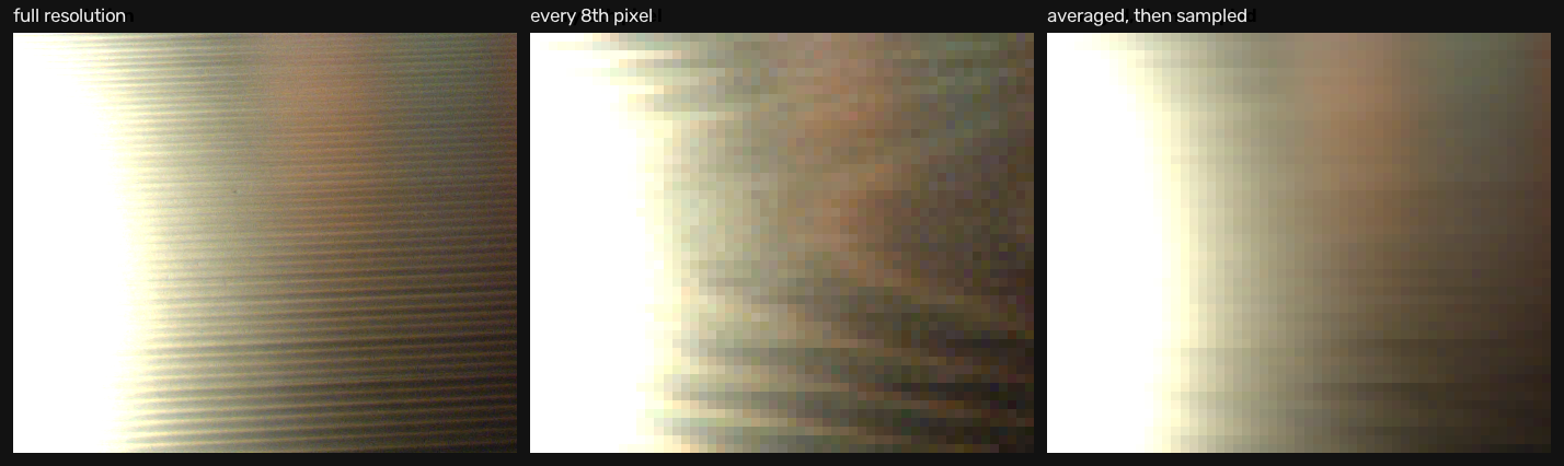
Lesson 2 of The Image as Data. One photosite on this camera is 5.527 µm and covers 1.056 arcminutes of the room. The table in the frame is ribbed at 7.4 pixels per cycle; keep every 8th pixel and it comes back at 96 pixels per cycle — thirteen times too coarse, and predicted exactly by folding the frequency.
TL;DR — one photosite on this camera is 5.527 µm across and covers 1.056 arcminutes of the room. The table in the frame is ribbed at 7.4 pixels per cycle. Keep every 8th pixel and that ribbing comes back at 96 pixels per cycle — thirteen times too coarse, and a pattern the room does not contain. Where it lands is arithmetic, and the measurement agrees with the arithmetic in every case.
Where we are
Part of The Image as Data. Lesson 1 left the array knowing what its numbers are and nothing about where they came from. This lesson is about the grid: how far apart the samples are, and what happens to whatever lies between them.
What one sample covers
Intuition: a photosite is a small square that collects everything falling on it, so a pixel is not a point measurement — it is an average over a patch of the world.
The D2X puts 4288 effective pixels across a 23.7 mm sensor [2], so
and the vertical pitch works out to 5.513 µm from the other side of the sensor — they agree to 0.014 µm, which is the check that the sensor is on a square grid. At this scene’s 18 mm focal length, one photosite subtends
What it means: roughly one arcminute per pixel, which is about the resolving limit of a good human eye. The chart’s white patch is sampled 2,916 times inside its measurement box alone. Its border is sampled once. Every error a grid makes lives at the edges, because that is the only place where one sample has to stand for two things.
The pattern that is finer than the grid
The table under the lamp is ribbed, and that ribbing is the only strongly periodic thing in the frame — which makes it the one place where sampling can be measured rather than asserted.
Measuring it turned up something the plan did not expect. The ribbing has no single period: it runs from 6.19 px per cycle at the far edge of the crop to 13.71 px at the near edge, monotonically.
| frame row | 2100 | 2196 | 2292 | 2388 | 2484 | 2580 | 2676 |
|---|---|---|---|---|---|---|---|
| period (px) | 6.19 | 7.38 | 8.00 | 9.60 | 10.67 | 12.00 | 13.71 |
That is not noise, it is perspective: a physical grating photographed at a shallow angle is foreshortened at the far end. So the frequency work below runs on a 192-row window — frame rows 2196 to 2388 — where the period is 7.385 px and roughly constant.
Where an undersampled pattern goes
Intuition: if you only look every -th pixel, a fast wiggle and a slow wiggle can produce the identical sequence of numbers, and nothing downstream can tell them apart.
Keeping every -th sample multiplies the frequency in the new grid by . Anything past half a cycle per sample has nowhere to go and reflects back:
| decimation | samples per cycle | apparent period | |
|---|---|---|---|
| every 2nd pixel | 3.69 | above Nyquist | 7.4 px — the truth |
| every 4th pixel | 1.85 | below | 8.7 px |
| every 8th pixel | 0.92 | below | 96 px |
In all three cases the measured peak falls in the bin the fold predicts. The bin is 0.010, 0.021 and 0.042 cycles per new pixel respectively — coarse at ×8, so the honest claim is “lands in the predicted bin”, not “exact to four decimals”.
What this costs when you resize
The fix is to average over the footprint before sampling, which is what
cv2.INTER_AREA does [4]. Measured against that reference on the ribbed crop:
| every 2nd | every 4th | every 8th | |
|---|---|---|---|
| nearest (bare sampling), RMS | 1.741 | 3.358 | 4.428 |
| bilinear — OpenCV’s default — RMS | 0.000 | 1.307 | 2.704 |
What it means: bilinear and area agree exactly at ×2, then diverge. INTER_LINEAR
is cv2.resize’s default and it reads only a 2 × 2 neighbourhood, so past ×2 it is
skipping most of the pixels it is supposed to be averaging. On the flat white patch,
where there is nothing above Nyquist to lose, the same ×4 comparison gives 1.874 and
0.963 — the methods barely differ. Aliasing is a property of the content, not of the
resize call.
small = cv2.resize(img, (w // 8, h // 8), interpolation=cv2.INTER_AREA)   # averages
naive = cv2.resize(img, (w // 8, h // 8), interpolation=cv2.INTER_NEAREST)  # samples
# INTER_LINEAR is the default and reads a 2x2 neighbourhood: fine at x2, not at x8.cv::Mat small, naive;
cv::resize(img, small, cv::Size(w / 8, h / 8), 0, 0, cv::INTER_AREA);
cv::resize(img, naive, cv::Size(w / 8, h / 8), 0, 0, cv::INTER_NEAREST);Now you try
Leave the period at the measured 7.385 px and walk the sampling interval up from 1. Nothing happens until you pass 3; then the reconstruction detaches from the signal completely. Now nudge the period to 7.4 — a change of 0.015 px — and the answer at ×8 moves from 96 px to 99. Folding multiplies any error in the period by the sampling interval, which is why the article names the window its 7.385 was measured in.
In the wild
Two of them, because this is the one lesson where a still picture cannot show the whole idea.
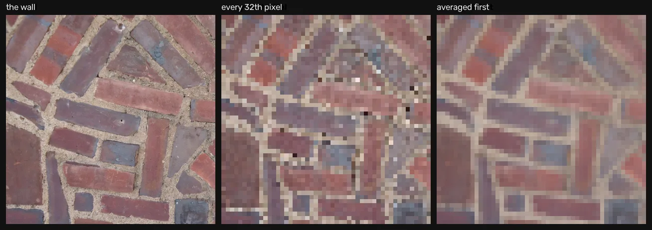
First, a brick wall — and the moment you make a thumbnail. Photographed square-on at 2592 × 1944, the courses of brick repeat every 54.0 pixels. That is enormous, so shrinking to 648 px or even 162 px is perfectly safe: 13.5 and 3.4 samples per cycle, both above the two that Nyquist asks for. Then:
| shrink to | width | samples per cycle | pattern you get back | |
|---|---|---|---|---|
| ÷16 | 162 px | 3.38 | above | 52.8 px — the wall |
| ÷32 | 81 px | 1.69 | below | 81.3 px |
| ÷64 | 40 px | 0.84 | below | 330.7 px |
What it means: 81 pixels wide is a thumbnail and 40 pixels is an avatar. Those are not exotic sizes — they are what a gallery grid and a comment avatar are, and they are exactly where a regular texture stops being itself. At ÷64 the wall comes back as a pattern six times too coarse, which is why brickwork and pinstripes look so strange in small previews.
Second, the version you cannot print. A grid samples space; a camera also samples time, and everything above applies to frames the same way it applies to pixels. Filmed at 24 frames per second, a spoked wheel turning forwards can be recorded turning backwards.

What it means: the sign is the finding. The wheel is not ambiguous and it is not blurred — it is confidently rotating the wrong way, and no processing of those frames can recover the truth, because the frames are consistent with the wrong answer. One honest limit: a spoke looks like the next spoke, so apparent rotation is only ever known modulo the 45° between them. That is the temporal twin of the 96-pixel ripple above.
Where this breaks
This lesson shows that undersampling substitutes one pattern for another, and gives the arithmetic for where the substitute lands. It does not explain why two samples per cycle is the threshold, or what “average first” is really doing. Both of those are statements about the frequency content of an image, and they belong to the frequency domain unit, which is not written yet. Taking the rule on trust here is deliberate.
Two more honest limits. The drift table means the “7.385 px” figure is one window’s value, not the table’s; a different crop gives a different period, and any conclusion that depends on the exact number has to name the window. And these code values are not proportional to light — unit 1.2 measured the curve that sits between them — so averaging code values is not averaging light. For a resize nobody notices; for photometry it matters.
Next
Quantization: how many bits a pixel deserves — the samples are in the right places now, so the question becomes how finely each one is allowed to be written down.
Further reading
- Go deeper: Gonzalez & Woods, Digital Image Processing (4th ed.), §2.4 (Image Sampling and Quantization, p. 47) [1] — Spatial and Intensity Resolution (p. 55) and Image Interpolation (p. 61) are the two subsections behind this lesson.
- Related on CondadosAI: what a raw count means · the response curve, which is why averaging code values is not averaging light.
References
[1] Gonzalez, R. C., & Woods, R. E. (2018). Digital Image Processing (4th ed.), §2.4 (Image Sampling and Quantization, p. 47), incl. Spatial and Intensity Resolution (p. 55) and Image Interpolation (p. 61). Pearson. Detailed table of contents.
[2] Nikon. D2X specifications — 23.7 × 15.7 mm CMOS, 12.4 million effective pixels, 4288 × 2848 image area. Product page.
[3] Fairchild, M. D. (2007). The HDR Photographic Survey. Proceedings of the IS&T 15th Color and Imaging Conference, pp. 233–238. doi:10.2352/CIC.2007.15.1.art00044 — the scene this unit measures. Used for research and non-commercial publication, as its terms require; images are downloaded, never redistributed.
[4] OpenCV. Geometric image transformations — resize and the interpolation flags, OpenCV 5.0.0 documentation. Docs.