How many good parts does it take to beat a System One AI model? Between one and sixteen, on VisA

TL;DR

• A “System One” AI model, the kind TypeSafe launched with Jev in September 2026, reads a photo and a question and returns a decision in one step. It can start inspecting products on the first day of a production line, with no examples. A specialised defect detector that learns from photos of good products overtakes it after one to sixteen of those photos per product. A line that starts with the System One model should collect good examples from the first shift.
• On the VisA benchmark (12 products, 2,162 test images), Jev-Omni, an open System One model, and the untouched Gemma 4 12B it was built from score a macro AUROC of 81.1 and 82.9 without seeing a good part. AUROC is a ranking score where 50 is a coin flip and 100 is perfect.
• PatchCore, the specialised detector, passes Jev-Omni with eight good parts per product and Gemma 4 with sixteen at anomalib’s default 256-pixel input, the plan I fixed before the run. At 512 pixels it needs one and four. The input size moves the answer more than the choice of general model does.
• Jev-Omni scores 1.8 points below its own base model read the same one-pass way (95% interval 0.8 to 2.8): here, with this prompt, the System One fine-tune cost accuracy.
• Once labelled parts are available to set the thresholds, a line where 1% of parts are defective and at most 5% of defects may get through can hand 36% to 39% of its parts to the general models and 70% to PatchCore with sixteen good parts at 512 pixels, with no person involved.
• On an unlabelled lime line, one sentence of product spec more than doubles how closely Gemma 4’s score follows the colour that grades limes; the threshold still needs labelled parts. About $6 of rented GPU in all.

What a System One model is

In September 2026 TypeSafe launched Jev and called it the first “System One model” [17]. The name comes from Daniel Kahneman’s split between fast, automatic System 1 thinking and slow, deliberate System 2 reasoning [18]. A chat model answers by writing text, one word at a time. A System One model answers with a decision instead: you give it a situation and a fixed list of options, and it returns one probability per option in a single pass, with no text to parse. TypeSafe describes Jev as “unstructured state in, typed probabilistic decisions out”, claims it is two orders of magnitude faster and more efficient than existing LLMs on such tasks, and launched it in early access [17].

That shape fits an inspection line well: a photo and “good or defective?” go in, a probability comes out, and no one has to collect examples of the product first. Jev launched in early access, so I tested the System One interface in two open forms. Both are vision-language models (VLMs), which take an image and a question in plain text. Used zero-shot, meaning as they come, with no example of the product, they can inspect a part from the first day.

	Jev-Omni [1]	Gemma 4 12B [2], read in one pass
What it is	Gemma 4 12B with fine-tuned weights and a trained decision head; open, not affiliated with TypeSafe	The same base model, untouched
How the answer is read	The head returns one probability per option	The probability that the next token is “1” or “2”
Trained for System One decisions	Yes	No
Where it appears in this post	The VisA benchmark	The VisA benchmark and the lime-line video, because it scored higher on VisA

Jev-Omni is built on Gemma 4, so testing both answers a practical question: does the System One training add anything on this task, or does reading the base model the same way already do the job?

What it looks like in Python

Jev-Omni ships its own loader, and one call returns a probability per option:

import sys
from huggingface_hub import snapshot_download

path = snapshot_download("akhilaaa3/Jev-Omni", revision="5addda86ddee081a68fb067477ea100c221b8917")
sys.path.insert(0, path)
from jev_omni import load_jev_omni

classifier = load_jev_omni()
result = classifier.predict(
    state="Production-line inspection photo of a cashew nut.",
    question="Is everything in the photo good, or is at least one part defective?",
    options=["all good", "defective"],
    media="cashew_anomaly_000.jpg",
    modality="image",
)
print({k: round(v, 3) for k, v in result["probabilities"].items()})
# {'all good': 0.39, 'defective': 0.61}

The untouched Gemma 4 needs a few more lines. The prompt lists the options as numbers and asks for the number only; the model runs once over the photo and the prompt; and instead of letting it write an answer, the code reads the probability it gives to “1” and to “2” as the next token and normalises the two:

import torch
from PIL import Image
from transformers import AutoProcessor, Gemma4UnifiedForConditionalGeneration

model_id, revision = "google/gemma-4-12B-it", "707f0a3b8a3c7ad586ed01e27eafbad8a27dd0f7"
processor = AutoProcessor.from_pretrained(model_id, revision=revision)
model = Gemma4UnifiedForConditionalGeneration.from_pretrained(
    model_id, revision=revision, dtype=torch.bfloat16, device_map="cuda")

options = ["all good", "defective"]
prompt = ("Production-line inspection photo of a cashew nut.\n\n---\n\n"
          "QUESTION: Is everything in the photo good, or is at least one part defective?\n\n"
          "OPTIONS:\n1. all good\n2. defective\n\n"
          "Reply with only the number of the correct option (1-2).\n"
          "Output a single number and nothing else.")
messages = [{"role": "user", "content": [
    {"type": "image", "image": Image.open("cashew_anomaly_000.jpg").convert("RGB")},
    {"type": "text", "text": prompt}]}]
inputs = processor.apply_chat_template(messages, add_generation_prompt=True, tokenize=True,
                                       return_dict=True, return_tensors="pt", enable_thinking=False)
inputs = inputs.to("cuda", dtype=torch.bfloat16)

with torch.inference_mode():
    logits = model(**inputs, logits_to_keep=1).logits[0, -1]  # one pass, nothing generated

digit_ids = [processor.tokenizer.convert_tokens_to_ids(str(i + 1)) for i in range(len(options))]
probs = torch.softmax(logits[digit_ids].float(), dim=0)
print({k: round(v, 3) for k, v in zip(options, probs.tolist())})
# {'all good': 0.029, 'defective': 0.971}

Both snippets are condensed from examples/system_one_readout.py in the companion repo, and the printed lines are what they returned on an L40S for the defective cashew Anomaly/000.JPG. They match the scores the benchmark saved for that photo. On this cashew both lean defective, the base model far more confidently. The benchmark then asks every question twice with the options swapped, for a reason the next sections explain.

This post puts both against the usual alternative in inspection: a detector that needs photos of good parts before it can work. The comparison a line engineer would make is between a model that works from the first part and one that works better once it has seen enough good parts. The number of good parts where the second one takes over is the useful answer, so that is the headline, and I fixed how it would be computed before running anything.

The comparison in one video

In the video below, thirteen VisA test parts stop one at a time under an inspection window. Two cards give the two systems’ verdicts, and then the true label appears.

1. A test photo comes up: one VisA part that neither system has seen.
2. Gemma 4 gets the photo and the question “is everything in the photo good, or is at least one part defective?”, with no example of a good part. PatchCore gets the same photo after storing 16 photos of good parts of that product.
3. Each returns a score. Gemma 4’s says how strongly it leans towards “defective”; PatchCore’s says how far the most unusual patch of the photo is from anything in the good photos. The magenta overlay marks those unusual patches.
4. Two cuts per product turn each score into accept, send to a person, or reject. The cuts let at most 5% of defective parts through and throw away at most 5% of good ones, the requirement the triage section below explains.
5. The true label from VisA appears last. I picked the thirteen parts by hand to show every outcome (both right, each one wrong), so the belt says nothing about rates: on it Gemma 4 accepts 4 of the 9 defective parts and PatchCore 1. The cuts were fitted on all test images of each product, these included, and every verdict is read from the saved scores.

The data: VisA

VisA [3] has 12 products photographed on a bench: four printed circuit boards, four products with several items per photo (candles, capsules, two kinds of macaroni) and four with one item (cashew, chewing gum, two fried snacks). Its official split gives each product between 450 and 905 good training images (I hold one of them out per product as the VLMs’ reference photo, so PatchCore draws from 449 to 904) and a test set of 50 to 101 good parts plus 100 defective ones. Every defective image carries a pixel mask (the kind scored in the segmentation metrics post) and one or more defect types (“small scratches”, “missing”, “similar colour spot”). The dataset is CC BY 4.0 [4].

Two properties of that test set matter later. It is 55% defective, where a real line runs at a percent or less, so every number that depends on the defect rate is reweighted below. And 100 defects per product is enough to rank systems but thin for rates of a few percent, so the triage numbers carry intervals.

Three ways to score a part

The first two are the System One readouts from the table above, Jev-Omni and Gemma 4 12B read in one pass. For the benchmark both get the same prompt, frozen before the run:

Production-line inspection photo of a cashew nut.

QUESTION: Is everything in the photo good, or is at least one part defective?

OPTIONS:
1. all good
2. defective

The object phrase is the only thing that changes per product (“macaroni pieces”, “a printed circuit board”). A second configuration adds one known-good photo of the same product before the test photo and says which is which; that puts the VLM on the same footing as PatchCore with one good part.

The score for AUROC and for thresholds is the log-odds of “defective” against “all good”. Log-odds is a confidence score: 0 means undecided, positive leans defective, negative leans good, and each step of +1 multiplies the odds of “defective” by about 2.7. A two-option readout leans toward one position, so every image is asked twice with the options swapped, and the two log-odds are averaged.

The swing has a direction. Averaged over all test images, listing “defective” second raises its log-odds by 0.41 for Jev-Omni and by 0.12 for the untouched Gemma 4. With a reference photo in front, the lean grows to 0.92 and 0.17. Averaging the two orders removes it from every number below.

PatchCore [5] works from good parts only. It remembers what small patches of good parts look like and flags a part when some patch looks like none of them. In detail, it runs each good image through an ImageNet-trained Wide ResNet-50 [7], keeps the feature vector of every image patch in a memory bank, and scores a test image by how far its most unusual patch is from the nearest patch in the bank. I used anomalib’s implementation [6] at its default settings, which resize every photo to 256 × 256, with k good parts per product for k = 1, 2, 4, 8, 16, 64 and all of them, each drawn at random three times (with fixed seeds, so anyone rerunning the code gets the same draws). The backbone weights are timm’s ImageNet-1k racm_in1k, anomalib’s default. After the main run I repeated k = 1, 4 and 16 at 512 × 512, for a reason the results section explains. 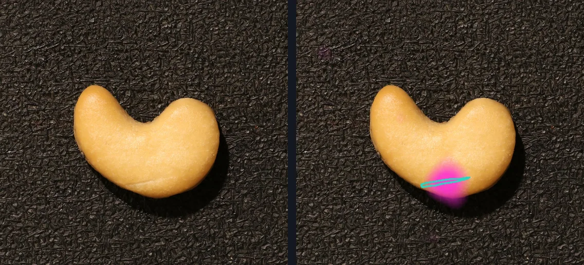Because the score is a distance per patch, PatchCore also says where the problem is:

Scoring the ranking: AUROC

The primary number is image AUROC per product, averaged over the 12 products with each counting the same (a macro average). AUROC asks one question: pick a defective part and a good part at random, how often does the system give the defective one the higher score? A coin scores 0.5 [9]. It ignores thresholds, which is what I want at this stage; the classification metrics post covers it alongside precision and recall, and Fawcett’s introduction [10] is the standard reference.

The pre-registered answer: eight good parts

The planned headline is k*, the smallest number of good parts at which PatchCore’s macro AUROC beats a VLM’s. “Beats” means the lower end of a 95% interval on the difference is above zero. A 95% interval is the range a number would likely land in if the test were rerun on other parts of the same products, so a range entirely above zero means PatchCore’s lead is unlikely to be luck of the draw. The interval comes from a paired bootstrap [11]: resample the good and the defective test images within each product, recompute both systems’ macro AUROC on the same resample, and for PatchCore also draw one of its three seeds, 2,000 times.

System	Good parts seen	Macro AUROC	95% interval
Jev-Omni, test photo only	0	81.1	79.4 – 82.7
Jev-Omni, reference + test photo	1	81.7	79.9 – 83.3
Gemma 4 zero-shot, test photo only	0	82.9	81.3 – 84.5
Gemma 4 zero-shot, reference + test photo	1	83.5	81.8 – 85.1
PatchCore, k = 1	1	80.8	78.0 – 83.1
PatchCore, k = 2	2	82.8	79.6 – 85.7
PatchCore, k = 4	4	83.6	80.2 – 86.5
PatchCore, k = 8	8	84.2	81.8 – 86.1
PatchCore, k = 16	16	85.7	84.2 – 87.2
PatchCore, k = 64	64	87.5	85.9 – 89.1
PatchCore, all (449–904)	all	90.2	89.0 – 91.4

The same sweep at 512 pixels

The two sides did not see the same image. Gemma 4’s processor turns each photo into 280 patches of 48 × 48 pixels, roughly 960 × 670 pixels of input; anomalib’s PatchCore sees 256 × 256. VisA photos are 1,274 to 1,562 pixels wide and many of its defects are a few pixels across (what a resize does to detail that small is the subject of the sampling post), so I reran the fast part of the sweep (k = 1, 4 and 16, three seeds each, everything else unchanged) at 512 × 512. This was not in the plan, and it is one extra setting tried once.

PatchCore, 512 px	Macro AUROC	95% interval	vs Jev-Omni	vs Gemma 4
k = 1	84.5	82.5 – 86.4	+3.4 [+1.0, +5.8]	+1.7 [−0.8, +3.9]
k = 4	89.7	88.1 – 91.4	+8.6 [+6.5, +10.9]	+6.8 [+4.7, +9.0]
k = 16	92.4	91.2 – 93.7	+11.3 [+9.4, +13.3]	+9.6 [+7.7, +11.4]

At 512 pixels, k* is 1 against Jev-Omni (also 1 against Jev-Omni with a reference photo) and 4 against Gemma 4 in both configurations. At k = 1, 4 and 16 the two resolutions are like for like (same draws, full memory bank), and 512 pixels adds 3.7 to 6.7 points at each of them. Sixteen good parts at 512 pixels (92.4) also score above every good part at 256 (90.2), but that last run differs in more than resolution: it subsamples its memory bank to 10%, has one seed, and the gap sits almost entirely in the group with several items per photo. I read the pre-registered eight as a property of the default resize as much as of the two methods. I tested one other size and no other backbone, so this shows that the input size matters a lot here and leaves open what the best PatchCore needs. I did not run k = 64 or all at 512: the coreset selection over several million patches per product takes hours, and that row is owed to a follow-up.

The 256-pixel run also produced a pattern by product type that I first took for a finding. At 256 pixels the ranking flips between circuit boards and products with several items per photo; at 512 pixels it mostly does not.

Group (products)	Jev-Omni, 0	Gemma 4, 0	PatchCore 1, 256 px	PatchCore 16, 256 px	PatchCore all, 256 px	PatchCore 16, 512 px
Circuit boards (4)	73.5	73.0	83.3	87.4	94.2	93.8
Several items per photo (4)	80.4	83.1	69.0	74.3	78.8	86.4
One item per photo (4)	89.3	92.6	90.1	95.4	97.7	97.1

On circuit boards, one good board at 256 pixels already gives PatchCore a 10-point lead: a board has the same layout every time, so any patch unlike the stored ones is suspicious. On capsules and macaroni1, which sit in different positions in every photo, the 256-pixel PatchCore stayed below Jev-Omni even with every good part (capsules 72.7 against 82.3, macaroni1 79.6 against 86.4), and I first read that as a real advantage of judging each item on its own. At 512 pixels, sixteen good capsules give PatchCore 90.1 and sixteen macaroni1 photos 90.8, so most of that gap goes away with resolution alone, in the one other size I tried. The one product where every system stays weak is macaroni2 (Jev-Omni 62.1, PatchCore 16 at 512 pixels 72.0).

A reference photo helps with missing parts

Adding a known-good photo changes the macro AUROC by less than a point for either VLM, but it moves specific defect types a lot. A missing component is the clearest case: to see that something is absent, you need to know it should be there.

On pcb1, pcb2 and pcb3, Jev-Omni goes from about chance on missing components (45, 54, 53) to 63, 71 and 82 with the reference in front, and the untouched Gemma 4 moves the same way (40, 50, 52 to 67, 75, 83). On pcb4, where missing parts are easier to see, it goes from 87 to 97 (33 images). The first three are 19 or 20 defective images each, from one run with one prompt, so they show a direction; the size of the effect is not measured. The last row runs the other way: on small scratches on cashews, Jev-Omni alone scores 31, below chance, meaning it rates scratched nuts as better than good ones, and the reference photo only lifts it to 53. On candles the same reference photo costs Jev-Omni 17 points (90.9 to 73.8), which I cannot explain from the images; it is one of the reasons the macro average barely moves.

Jev-Omni scores below its base model

Jev-Omni’s card reports accuracy on two decision benchmarks (DecisionBench and JevBench), on MMAU for audio and on MVBench for video, and on no image benchmark [1]. On VisA, Jev-Omni as shipped (fine-tuned weights plus head) is behind the untouched Gemma 4: 81.1 against 82.9 macro AUROC, a difference of −1.8 with a 95% interval of −2.8 to −0.8. Product by product, three differences survive a Holm correction [12], which raises the bar because 12 products were tested at once and one of them could look different by chance: cashew (−10.5), macaroni2 (−7.0) and candle (−4.4), each with an adjusted p-value of at most 0.006 (the floor of 2,000 resamples). None goes the other way significantly. The plan listed this comparison as descriptive, so it is a secondary finding, and it is a result about fit: the tasks Jev-Omni’s card reports are decision, audio and video benchmarks, none on images, and its open weights are what made this comparison possible in the first place. I compared the model as shipped with its base model and did not separate the fine-tune from the readout, and I used one prompt, so I cannot say which of the two costs the points.

From ranking to a line: triage

AUROC ranks; a line needs decisions. A common setup has three outcomes: accept parts that score low, reject parts that score high, and send the ones in between to a person. Two thresholds set how much each outcome gets. I fixed them the way a quality engineer would state a requirement: let through at most 5% of defective parts (escapes), and throw away at most 5% of good parts (overkill). Everything between the two cuts goes to a person. The thresholds are fitted per product, as a line would, by five-fold cross-fitting, so no image is judged by thresholds that saw it. Those thresholds are fitted on labelled test parts, 40 to 81 good and 80 defective per product and fold, for every system, including the zero-shot ones and PatchCore with one good part. No line has those labels on day 0, so the triage numbers describe what each score allows once labels exist.

The share of parts decided without a person depends on how many parts are defective. With a defect rate $\pi$:

$\text{coverage} = \pi \cdot P(\text{auto}\mid\text{defective}) + (1-\pi) \cdot P(\text{auto}\mid\text{good})$

Across all 12 products, on the held-out folds, escapes land between 4.3% and 4.9% and good parts rejected between 4.8% and 5.5%, close to the 5% the fitting folds were held to:

System	Escapes	Good parts rejected	Decided without a person, 1% defective
Jev-Omni, 0 good parts	4.8%	5.1%	36.3%
Gemma 4 zero-shot, 0	4.5%	4.9%	36.8%
Gemma 4 zero-shot, reference photo	4.3%	4.8%	39.2%
PatchCore, 1 good part	4.8%	5.1%	44.3%
PatchCore, 16	4.8%	5.5%	54.3%
PatchCore, all	4.7%	5.2%	66.2%
PatchCore, 16 at 512 px	4.8%	4.9%	70.3%

The triage ranking follows the AUROC ranking, including the resolution effect: sixteen good parts at 512 pixels decide more of the line than every good part at 256. PatchCore with a single good part and the untouched Gemma 4 cannot be told apart on AUROC ($-2.1$, interval $-5.1$ to $+0.8$), yet PatchCore decides more of the line. Triage at 5% escapes depends on the few lowest-scoring defects, a tail that AUROC averages away.

A zero-shot model’s scores look as if they should need no per-product threshold, since every product gets the same question and the same log-odds scale. In practice they need one: with a single pair of thresholds for all 12 products, the VLMs decide 18% to 23% of the line instead of 36% to 39%.

Now you try

Pick a system, then drag the two cuts on real scores for all 150 cashew test images. Watch how many defects slip through as you move “accept” to the right, and how the share sent to a person changes when you move the defect rate. The reset button fits the 5% cuts on all 150 images at once, without cross-fitting, so its numbers sit slightly off the worked example above (4 escapes instead of 6 for Jev-Omni).

Day 0 on a real line

VisA answers the question on a benchmark. To see what the zero-shot side looks like on footage nobody has labelled, I took a stock clip of a lime-sorting line [16] and built what a line could run on its first day: find each lime, follow it, crop it, ask Gemma 4 (the better of the two VLMs on VisA), and count the verdicts as the limes cross a line.

Limes that turn yellow are sorted out of export grade, and nothing in the frozen VisA question says so. I asked twice: once with the frozen question and “a lime”, and once with one sentence of product spec added (“Export grade requires a green skin; yellowing, spots or damage count as defects.”). With no labels to check the answers against, I measured each crop’s skin colour (median hue, where lower is yellower) and compared it with the score. Spearman’s ρ measures how consistently one goes up as the other goes down or up, from −1 to +1, with 0 meaning no relation; negative here means yellower limes get higher defect scores:

Prompt	Spearman ρ, score against hue	Flagged at P(defective) > 0.6
Frozen VisA question	−0.23 (p = 0.008)	83 of 128
With the one-sentence spec	−0.52 (p < 10⁻⁹)	126 of 128

The sentence more than doubles how closely the score follows skin colour, which is what a model you can talk to offers on day 0. It also pushes almost every lime past P = 0.6: the score puts the limes in an order you can check by eye, but its probability is not calibrated for this product. For the video I set two cuts on the score by eye, on this same clip.

The video runs at half speed. Boxes follow each lime and turn OK, PERSON or REJECT once Gemma 4 has judged it; the counters at the top go up as limes cross the dashed line.

1. Detect. RF-DETR [14], the detector family measured in the RF-DETR benchmark, draws a box around every round object in each frame. It was trained on COCO, which has no lime class, so it labels the limes “sports ball” with low confidence. That is enough to find round objects, so the detection threshold is set low.
2. Track. ByteTrack [15] links boxes across frames so each lime keeps one ID (the tracking metrics post covers how trackers are scored). It weighs box overlap by detection confidence, so the low COCO scores are stretched before tracking; the order of the detections does not change.
3. Crop before the line. For each lime I keep its largest clear view before it reaches the line and grey out everything outside an ellipse around it, so a neighbour’s blemish cannot answer for it. On a real line the decision has to exist before the part reaches the ejector.
4. Ask. The crop goes to Gemma 4 zero-shot with the question and the spec sentence. The answer is a score, the log-odds of “defective”.
5. Decide. A score below 6 is OK, above 10 is rejected, and anything in between goes to a person. I set these two cuts by eye on this clip.
6. Count. When a lime’s box crosses the dashed line, its verdict’s counter goes up by one.

The clip has no labels and the cuts come from the clip itself, so the video illustrates the pipeline and measures nothing. Setting those cuts properly needs labelled parts, good and defective, which is what the triage section used on VisA. A line that starts with a VLM on day 0 is therefore collecting labels from the first shift, and on VisA the same Gemma 4 readout is passed by PatchCore after four to sixteen good parts.

Reproducibility

Parameter	Value
Hardware	RunPod Secure Cloud, 1× NVIDIA L40S 48 GB, driver 580.126.09; CPU model, vCPU count and RAM were not recorded for this pod; no iGPU used
OS	Ubuntu 24.04 (image runpod/pytorch:1.0.3-cu1281-torch291-ubuntu2404)
Key versions	torch 2.14.0, torchvision 0.29.0, transformers 5.17.0, anomalib 2.6.2, timm 1.0.30, scikit-learn 1.9.1, numpy 2.5.3 (full list in results/pip-freeze.txt)
Models	Jev-Omni akhilaaa3/Jev-Omni @ 5addda86 (Apache-2.0) [1]; Gemma 4 google/gemma-4-12B-it @ 707f0a3b (Apache-2.0) [2]; PatchCore from anomalib 2.6.2 in fp32 with timm’s ImageNet-1k wide_resnet50_2.racm_in1k weights (Apache-2.0); sanity anchor wide_resnet101_2.tv_in1k (BSD-3-Clause)
Data	VisA [3], archive VisA_20220922.tar (sha256 2eb8690c…f362), official 1cls split: 2,162 test images (962 good, 1,200 defective)
VLM settings	bf16, batch 1, one forward per (image, configuration, option order); 8,648 per model. Our input path matches Jev-Omni’s own predict() to 2.4 × 10⁻⁸
PatchCore settings	256 × 256 input, no crop, layers 2+3, 9 neighbours; full memory bank for k ≤ 64, coreset ratio 0.1 for all; k-subsets nested, 3 seeds (1 for all, whose training set is fixed)
Statistics	macro AUROC, paired stratified bootstrap (2,000 resamples, seed 0); triage by 5-fold cross-fitting within product; Holm across 12 products
Command	bash scripts/pod_run.sh, then uv run jev-inspection score, scripts/ablation_summary.py, scripts/post_data.py and scripts/post_figures.py
Resolution ablation	PatchCore at 512 × 512, k = 1, 4, 16 × 3 seeds, on RunPod 1× L40 48 GB (driver 595.91.07), bash scripts/pod_ablation.sh; resize moved to the GPU for speed, identical to the CPU path to 1.1 × 10⁻⁶ per pixel
Day-0 demo	Pexels clip 32953325, 1080 × 1920 at 60 fps, every second frame (sha256 2bec11f3…1d72); RF-DETR base 1.11.0 (Apache-2.0), COCO classes sports ball, orange and apple at 0.05, class-agnostic NMS at 0.5, scores ×5 before ByteTrack (supervision, which multiplies IoU by the score when matching); counting line at 62% of the height; ellipse-masked crops ≥ 60 px taken before the line; Gemma 4 as above, both option orders; hue = median HSV hue of crop pixels with saturation > 0.35; scripts/demo_detect.py, demo_classify.py, render_counting_video.py. Illustrative, unlabelled
System One example	python examples/system_one_readout.py cashew_anomaly_000.jpg, same revisions as above, run on an L40S; output as printed in the post
Runs	one run per configuration; no latency is reported in this post (timings were logged and are in the per-image files)
Cost	L40S session 4 h 52 min (about $5.35), the L40 ablation (about$0.30) and short sessions for the demo videos (about $0.45)

The pre-registration, including the frozen prompt and the reasons for each departure from it, is in the repository’s DESIGN.md; the prompt and the scorer were committed on 25 September, before the run. The measured numbers are in results/: summary.json and summary_r512.json (AUROC, k*, triage, per-product and per-defect breakdowns), post_numbers.json (the worked examples), anchor.json, jev_equivalence.json, contamination_probe.jsonl, the per-image score files (the heat-map caption) and demo-limes/ (the day-0 video and its hue table). Costs, run times and driver versions come from the pod logs, and Gemma 4’s input size from its processor, as recorded in DESIGN.md.

Limitations

• The headline depends on a preprocessing setting. k* is 8 at anomalib’s 256-pixel default and 1 at 512 pixels. Both are single configurations, and I tried no other backbone, layer choice or input size, so neither number is the last word on how many good parts PatchCore needs.
• Our PatchCore is weaker than the published one, and I cannot say why. With a Wide ResNet-101 and all good parts at 256 pixels, my run scores 90.5; EfficientAD reports 94.3 for PatchCore on VisA [8], using the same backbone at 224 pixels, a 1% coreset, no crop and the authors’ own code (their Appendix B.5). My run had more pixels and a larger coreset, so the gap is not resolution. The candidates I have not checked are anomalib’s implementation against the original code and the backbone weights (timm’s against torchvision’s).
• The 512-pixel k* = 1 rests on three draws of a single good image per product. Another three draws could move it either way.
• One prompt. The VLM numbers come from one wording, averaged over two option orders. A better prompt could move them, in either direction. The reference-photo configuration also gives Jev-Omni’s head two images, an input it was not trained on, and uses one reference photo per product.
• The reference-photo results rest on 19–20 images per defect type and one run.
• VisA has been public since 2022. Gemma 4 may have seen it in training. Asked to name the dataset for 50 test images, it never said VisA (its most common answer was Food-101). That shows the model does not recognise the images and says nothing about whether it saw them in training.
• VisA is a bench. VisA photos are well lit, centred and still. A real line adds motion blur, lighting drift and parts that are only partly in view, all of which I did not test.
• Jev itself is not tested. It launched in early access; Jev-Omni offers the same interface but is a different model, trained by someone else, so these numbers say nothing direct about Jev.
• Speed is not reported here. Whether any of this runs at line rate, and on what hardware, is the subject of the next post.

What this means for a line

• With no data, a System One model is a reasonable start. It needs a photo and a sentence, and on VisA it ranked defects well above chance (macro AUROC 81 to 83) from the first part.
• Collect good parts from the first shift. A detector that learns from them caught up with the VLMs after one to sixteen photos per product (one to eight against Jev-Omni, four to sixteen against Gemma 4, depending on the input size) and kept improving.
• Write down what counts as a defect. On the lime line, one sentence of spec changed what the VLM ranked as defective.
• Plan for labels before automating decisions. Accepting and rejecting parts needs thresholds, and thresholds need labelled good and defective parts, for VLMs too. With them, and one threshold pair per product, PatchCore with sixteen good parts at 512 pixels decided 70% of the line against 36% to 39% for the VLMs, at the same escape rate.
• Check what each system sees. Shrinking the photos to 256 pixels changed the answer more than switching VLMs did.
• Here, the base model beat the fine-tune. Jev-Omni scored below the untouched Gemma 4 on this task, with this prompt; a zero-shot inspector from this family should start from the base model.
• What this does not tell you: how either system behaves on a real line, with motion blur, changing light and parts partly in view, or how fast it runs. The next post covers speed.

Further reading

• Go deeper on the statistics: Efron and Tibshirani’s An Introduction to the Bootstrap [11], for the percentile intervals used for every range in this post.
• The detector: the PatchCore paper [5], whose memory-bank argument is short and worth reading in full, and the anomalib documentation [6] for running it.
• Related on CondadosAI: the classification metrics post for ROC, precision and recall, and tracking metrics for how the tracker behind the day-0 video would be scored.

References

[1] akhilaaa3. Jev-Omni (model card, revision 5addda86). Hugging Face, 2026. huggingface.co

[2] Google DeepMind. Gemma 4 12B IT (model card, revision 707f0a3b). Hugging Face, 2026. huggingface.co

[3] Zou, Y., Jeong, J., Pemula, L., Zhang, D., & Dabeer, O. (2022). SPot-the-Difference Self-Supervised Pre-training for Anomaly Detection and Segmentation. ECCV 2022. arXiv:2207.14315 · DOI:10.1007/978-3-031-20056-4_23

[4] Amazon Science. spot-diff: the VisA dataset (README and LICENSE-DATASET, CC BY 4.0; commit 2a692ab5). GitHub, 2022. github.com

[5] Roth, K., Pemula, L., Zepeda, J., Schölkopf, B., Brox, T., & Gehler, P. (2022). Towards Total Recall in Industrial Anomaly Detection. CVPR 2022. arXiv:2106.08265 · DOI:10.1109/CVPR52688.2022.01392

[6] Akcay, S., Ameln, D., Vaidya, A., Lakshmanan, B., Ahuja, N., & Genc, U. (2022). Anomalib: A Deep Learning Library for Anomaly Detection. ICIP 2022, 1706–1710. arXiv:2202.08341 · DOI:10.1109/ICIP46576.2022.9897283. Documentation used: anomalib 2.6.2, PatchCore. anomalib.readthedocs.io

[7] Zagoruyko, S., & Komodakis, N. (2016). Wide Residual Networks. BMVC 2016. arXiv:1605.07146 · DOI:10.5244/C.30.87

[8] Batzner, K., Heckler, L., & König, R. (2024). EfficientAD: Accurate Visual Anomaly Detection at Millisecond-Level Latencies. WACV 2024, Table 2 and Appendix B.5. arXiv:2303.14535 · DOI:10.1109/WACV57701.2024.00020

[9] Hanley, J. A., & McNeil, B. J. (1982). The meaning and use of the area under a receiver operating characteristic (ROC) curve. Radiology, 143(1), 29–36. DOI:10.1148/radiology.143.1.7063747

[10] Fawcett, T. (2006). An introduction to ROC analysis. Pattern Recognition Letters, 27(8), 861–874. DOI:10.1016/j.patrec.2005.10.010

[11] Efron, B., & Tibshirani, R. J. An Introduction to the Bootstrap. Chapman & Hall/CRC, 1994, ch. 13 (Confidence Intervals Based on Bootstrap Percentiles). DOI:10.1201/9780429246593

[12] Holm, S. (1979). A Simple Sequentially Rejective Multiple Test Procedure. Scandinavian Journal of Statistics, 6(2), 65–70. JSTOR:4615733

[13] Clopper, C. J., & Pearson, E. S. (1934). The use of confidence or fiducial limits illustrated in the case of the binomial. Biometrika, 26(4), 404–413. DOI:10.1093/biomet/26.4.404

[14] Robinson, I., Robicheaux, P., Popov, M., Ramanan, D., & Peri, N. (2026). RF-DETR: Neural Architecture Search for Real-Time Detection Transformers. ICLR 2026. arXiv:2511.09554 · GitHub

[15] Zhang, Y., Sun, P., Jiang, Y., et al. (2022). ByteTrack: Multi-Object Tracking by Associating Every Detection Box. ECCV 2022. arXiv:2110.06864

[16] Comercial GB. Lime sorting on conveyor belt in factory. Pexels video 32953325, Pexels licence. pexels.com

[17] Almeida, D. (2026). Introducing System One Models & Jev. TypeSafe AI blog, 15 September 2026. typesafe.ai

[18] Kahneman, D. (2011). Thinking, Fast and Slow. Farrar, Straus and Giroux, Part I (Two Systems).