
Why it works: Unit 1.2: Image sensing, Unit 1.3: The image as data
Fix a Badly Exposed Photo with OpenCV
The first OpenCV in Practice project: open a photo taken two stops too dark, read its histogram, try five ways to fix it, and measure each against a longer, better-exposed shot of the same scene (the target). Multiplying lands closest; the automatic fixes land furthest.

A photo taken with too little light can often be brightened to look like a longer exposure of the same scene, and this project measures which way of brightening gets closest.
The animation turns a single setting up, the multiplier applied to every pixel, and shows the fixed photo next to a longer, better-exposed shot of the same scene (the target), with the gap between them counting down.
- Open the photo. Load the file into a grid of numbers, one per colour per point (lesson 1).
- Read its histogram. Count how many pixels sit at each brightness, which shows how dark the photo is and what is already burnt out (lesson 2).
- Fix the exposure. Change every value by one rule: add a constant, multiply by a gain, bend with a gamma curve, or let an automatic equalizer decide (lessons 3, 4 and 5).
- Measure the gap. Compare the fixed photo with a longer, better-exposed shot of the same scene (the target), pixel by pixel, and average the difference. Lower is closer; 0 is identical.
- Crop, resize, save. Keep the part you want, shrink it without aliasing, and write it to a file (lesson 6).
Where you have met it: the Exposure and Brightness sliders in phone photo editors and in Lightroom; the Auto button next to them; the histogram on a camera’s playback screen.
TL;DR. Brightening a dark photo by scaling its values gets far closer to the target exposure than adding to them or letting an automatic tool decide, and nothing brings back what the camera burnt out. Two stops dark (almost a quarter of the light the target got), a gain of 2.4 leaves an average gap of 9.1 (out of 255) to the target, adding brightness 18.0, and histogram equalization 30.6. Three stops dark, gamma wins, 13.9 against 15.1.
The scene and the target
Every lesson works on one scene: a desk lamp, a card and a colour chart, photographed eighteen times at shutter times from 1/800 s to 30 s for Mark Fairchild’s HDR Photographic Survey [1]. Unit 1.2 of the Fundamentals track measures the same eighteen raw files. This module uses four, developed the same way:
| File | Shutter | Mean grey | Grey ≥ 250 | Role |
|---|---|---|---|---|
reference.webp | 5 s | 104.7 | 11.7% | the target every fix is scored against |
dark.webp | 1.3 s | 56.6 | 7.8% | about two stops under |
darker.webp | 1/2 s | 40.8 | 6.3% | more than three stops under |
bright.webp | 20 s | 173.8 | 27.2% | two stops over |
The distance used throughout is the mean absolute difference between the fixed photo and the target, over every pixel and colour channel, on the 0–255 scale.
The whole fix, in one cell
import cv2
import numpy as np

img = cv2.imread("dark.webp")
ref = cv2.imread("reference.webp")

fixed = cv2.convertScaleAbs(img, alpha=2.4)
gap = np.abs(fixed.astype(int) - ref.astype(int)).mean()
print("distance to the reference:", round(gap, 1))

cv2.imwrite("fixed.jpg", fixed, [cv2.IMWRITE_JPEG_QUALITY, 90])
side = [cv2.resize(x, None, fx=0.5, fy=0.5) for x in (img, fixed, ref)]
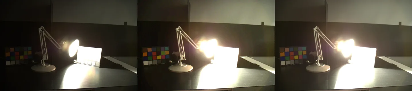
cv2.imshow("dark | fixed | reference", np.hstack(side))distance to the reference: 9.1
What each fix gets
Each fix was scored at its best setting, found by trying its parameter in small steps (values in brackets).
| Fix | Dark, 1.3 s | Darker, 1/2 s | Bright, 20 s |
|---|---|---|---|
| nothing | 47.0 | 62.3 | 68.4 |
| add a constant (value) | 18.0 (50) | 25.7 (65) | 68.4 (0) |
| multiply (gain) | 9.1 (2.4) | 15.1 (4.2) | 22.8 (0.5) |
| gamma (γ) | 10.7 (0.55) | 13.9 (0.4) | 33.4 (2.35) |
equalizeHist on brightness | 30.6 | 31.9 | 30.3 |
| CLAHE on brightness | 35.5 | 51.3 | 58.8 |
Four things come out of the table:
- A gain beats an offset. A longer exposure multiplies the light, so a multiplier is the right shape of fix, and it halves the gap that adding leaves (lesson 3). OpenCV’s own tutorial warns that the offset leaves a grey veil [3].
- Gamma overtakes the gain as the photo gets darker. A gain large enough to lift three stops of shadow pushes everything above 60 to white; gamma maps 0 to 0 and 255 to 255 at every setting, so it never clips [2] (lesson 4).
- The automatic fixes land furthest. Equalization spreads brightness by how common each level is [2], and this photo is mostly dark wall and desk (lesson 5).
- Overexposure is the hard direction. Nothing gets the bright photo closer than 22.8, because 15.6% of its pixels are at 250 or above where the target still has detail. Those values are gone.
What to take from it
- A photo a stop or two dark: multiply by one gain and check it against something you trust (a grey card, a second shot). Here that closed 47.0 to 9.1.
- Much darker than that: use gamma instead, or a gain and gamma together, and accept flatter shadows. Here 62.3 went to 13.9.
- No reference and you only need to see detail: equalization or CLAHE, knowing the result will not look like the scene.
- Overexposed: re-shoot or bracket. Software got the bright photo only to 22.8, and 15.6% of it could not be recovered by any setting. High dynamic range shows how several exposures of this scene are merged to keep everything.
- When a model is worth it: this module did not test a learned enhancer. The number to beat is 9.1 two stops down and 13.9 three stops down.
Limitations
- The target is a choice, not the truth. The 5-second shot already has 11.7% of its pixels at 250 or above. The dark photo kept detail in the lamp that the target lost, so a fix that preserved it is scored as worse.
- The best settings were picked by looking at the answer. Every gain and gamma above was chosen to minimise the distance to the target. Without a target you would have to choose by eye or by a rule, and do worse.
- One scene, one camera. A lamp in a dark room is an extreme range of light. A flatter scene would favour equalization more, and the order of the fixes could change.
- The distance weighs every pixel equally. Most of this frame is dark wall and desk, so the score mostly reflects the shadows. A metric that weighted the lamp and chart more would rank the fixes differently.
- The inputs are WebP at quality 90. Every number was computed from the published files, so a reader’s Run reproduces it, but they are not the raw sensor values.
The lessons
- Open an Image and Read Its Pixels in OpenCV
- Image Histograms in OpenCV
- Brightness and Contrast in OpenCV
- Gamma Correction in OpenCV with a Lookup Table
- Histogram Equalization and CLAHE in OpenCV
- Crop, Resize and Save an Image in OpenCV
Every cell of the module is also in one notebook, to run on your own machine with the OpenCV pip installs: open it in Colab. Its outputs match the page’s, cell for cell.
How these numbers were made
| Data | HDR Photographic Survey, “Luxo Double Checker” [1]: files _MDF0010.NEF (1/2 s), _MDF0011.NEF (1.3 s), _MDF0013.NEF (5 s), _MDF0015.NEF (20 s). Research and non-commercial terms; downloaded, not redistributed as raw |
| Development | rawpy 0.27.0 (LibRaw 0.22.1): camera white balance, no auto-brightening, half size, 8-bit; resized to 960 px wide with INTER_AREA; written as WebP quality 90 |
| Scores | Mean absolute difference to reference.webp over all pixels and channels. Grids: add 0–150 in steps of 5; gain 0.2–6.0 in steps of 0.1; gamma 0.20–3.00 in steps of 0.05; CLAHE clipLimit=2.0, tileGridSize=(8, 8) |
| In the page | Pyodide 314.0.7, OpenCV 4.11.0, NumPy 2.4.6 (every cell’s shown output is rendered by npm run pycells with this build) |
| Locally | OpenCV 5.0.0, NumPy 2.5.2, Python 3.12; every number in the table above matches the page’s to one decimal |
| Machine | Intel Core i7-12700H, Ubuntu 22.04.5 LTS. Nothing is timed; the numbers are deterministic |
| Commands | uv run --extra sensing sensing-download, then uv run --extra sensing practice-m1 --assets --media in fundamentals-lab; npm run pycells in the site repo |
| Artifact | output/practice_m1_numbers.json |
Further reading
- Gonzalez & Woods, Digital Image Processing, chapter 3 [2], for intensity transformations and histogram processing with the theory behind each.
- OpenCV’s tutorial Changing the contrast and brightness of an image! [3], which corrects a different underexposed photo with α, β and γ.
- Image sensing, the Fundamentals unit on this same scene, for why the camera clipped where it did and how the eighteen exposures merge into one.
References
[1] Fairchild, M. D. (2007). The HDR Photographic Survey. IS&T 15th Color Imaging Conference, pp. 233–238. doi:10.2352/CIC.2007.15.1.art00044
[2] Gonzalez, R. C., & Woods, R. E. (2018). Digital Image Processing (4th ed.), chapter 3 “Intensity Transformations and Spatial Filtering”: section 3.2 “Some Basic Intensity Transformation Functions”, p. 136, and section 3.3 “Histogram Processing”, p. 147. Pearson.
[3] OpenCV. Changing the contrast and brightness of an image! (tutorial, doc/tutorials/core/basic_linear_transform/basic_linear_transform.markdown). OpenCV 4.11.0, commit 31b0eee. github.com/opencv/opencv