
Why it works: Unit 1.2: Image sensing, Unit 1.3: The image as data
Image Histograms in OpenCV
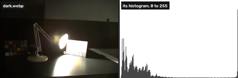
Count how many pixels sit at each brightness with cv2.calcHist, draw the histogram, and read from it that the dark photo has 79.3% of its pixels in the bottom quarter and 7.8% burnt out.
A histogram counts how many pixels have each brightness, which tells you at a glance whether a photo is too dark, too bright or both.
Where you have met it: the histogram on a camera’s playback screen and in a phone camera’s pro mode; the histogram panel in Lightroom, darktable and GIMP’s Levels dialog.
TL;DR. A histogram shows where a photo’s brightness sits, so you can see a bad exposure before you fix it. In the dark photo, 79.3% of the pixels sit in the bottom quarter of the range and 7.8% are at 250 or above, which means it is too dark and burnt out at the same time.
The problem
Lesson 1 summed the photo up in one number, a mean brightness of 56.6. A mean hides the shape: a photo that is half black and half white also averages near 128. To decide how to fix the exposure you need the whole distribution.
Count the pixels at each brightness
cv2.calcHist takes a list of images, the channel to count, an optional mask, the number of bins and the range of values [1]. With 256 bins over [0, 256], each bin is one grey level.
import cv2
import numpy as np

img = cv2.imread("dark.webp")
grey = cv2.cvtColor(img, cv2.COLOR_BGR2GRAY)
hist = cv2.calcHist([grey], [0], None, [256], [0, 256])

low = 100 * hist[:64].sum() / grey.size
high = 100 * hist[250:].sum() / grey.size
print("darkest quarter (0-63):", round(low, 1), "%")
print("250 or above:", round(high, 1), "%")darkest quarter (0-63): 79.3 % 250 or above: 7.8 %
| Argument | Here | What it means |
|---|---|---|
[grey] | one image | a list, because it can count across several images |
[0] | channel 0 | the only channel of a grey image |
None | no mask | pass a mask to count only part of the image |
[256] | 256 bins | one per grey level |
[0, 256] | the range | the upper end is not included |
Nearly four pixels in five sit in the darkest quarter. That is the underexposure. The 7.8% at 250 or above is the lamp and the pool of light under it, which were already too bright at this exposure: no amount of brightening will bring detail back there.
Draw it
A histogram is easier to read as a picture. The function below draws one bar per grey level with cv2.line, then puts the dark photo’s histogram beside the target exposure’s.
def draw_histogram(grey, height=200):
    hist = cv2.calcHist([grey], [0], None, [256], [0, 256]).ravel()
    canvas = np.full((height, 256, 3), 255, np.uint8)
    for value, count in enumerate(hist / hist.max()):
        top = int(height * (1 - count))
        cv2.line(canvas, (value, height), (value, top), (80, 80, 80))
    return canvas

ref = cv2.cvtColor(cv2.imread("reference.webp"), cv2.COLOR_BGR2GRAY)
cv2.imshow("dark (left) and reference (right)",
           np.hstack([draw_histogram(grey), draw_histogram(ref)]))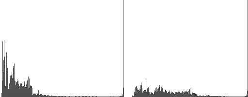
The target’s histogram is spread across the whole range. The dark photo’s is squashed into the left end. The fixes in lessons 3, 4 and 5 are three different ways of stretching the left histogram toward the right one, and this picture is what they are all trying to reach.
Break it
The range is half-open: [0, 256] counts 0 through 255. Writing [0, 255], the natural-looking version, silently drops every pixel at 255.
# The range excludes its upper end: [0, 255] drops 255
wrong = cv2.calcHist([grey], [0], None, [256], [0, 255]).ravel()
right = cv2.calcHist([grey], [0], None, [256], [0, 256]).ravel()
print("pixels at 255, range [0, 255]:", int(wrong[255]))
print("pixels at 255, range [0, 256]:", int(right[255]))pixels at 255, range [0, 255]: 0 pixels at 255, range [0, 256]: 41503
41,503 pixels, the burnt-out lamp, vanish from the count, and nothing warns you. The mistake is easy to pick up from OpenCV’s own tutorial, whose text gives the range as [0,255] [1] while its sample code passes (0, 256) with the comment “the upper boundary is exclusive” [4].
Your turn
The overexposed photo, bright.webp, was taken at 20 seconds. What percentage of its grey pixels are at 250 or above? Store the answer in clipped.
# percent of grey pixels at 250 or above in bright.webp
clipped = 0.0
print(clipped)
Why this works
A histogram is the distribution of intensity values [2]. It says nothing about where in the frame the pixels are, only how many of each value there are, which is why two very different photos can share one. Why the lamp clips at one end while the desk is lost in the dark at the other is a property of the sensor: Noise and dynamic range measures how wide a range one exposure can hold, and High dynamic range shows how several exposures of this same scene are merged to hold all of it.
Common mistakes
[0, 255]as the range. It drops the value 255, as the Break it cell shows.- Passing the image instead of a list.
calcHist(grey, …)fails; it must becalcHist([grey], …). - A colour image with channel
[0]. That counts only the blue channel. Convert to grey first, or count each channel on purpose. - Reading bar heights as percentages.
calcHistreturns counts. Divide bygrey.sizefor fractions. - Indexing the result as
hist[v, 0]. OpenCV 4.11 returns a column of shape (256, 1), OpenCV 5.0 a flat array of shape (256,), so that index works on one and fails on the other (both checked on 30 Sep 2026). Call.ravel()first, as the cells here do.
References
[1] OpenCV. Histogram Calculation (tutorial, doc/tutorials/imgproc/histograms/histogram_calculation/histogram_calculation.markdown). OpenCV 4.11.0, commit 31b0eee. github.com/opencv/opencv
[2] Gonzalez, R. C., & Woods, R. E. (2018). Digital Image Processing (4th ed.), section 3.3 “Histogram Processing”, p. 147. Pearson.
[3] Fairchild, M. D. (2007). The HDR Photographic Survey. IS&T 15th Color Imaging Conference, pp. 233–238. doi:10.2352/CIC.2007.15.1.art00044
[4] OpenCV. samples/python/tutorial_code/Histograms_Matching/histogram_calculation/calcHist_Demo.py, line 27. OpenCV 4.11.0, commit 31b0eee. github.com/opencv/opencv