Boundary Detection: Finding Lines and Circles with the Hough Transform

This unit is about finding straight lines and circles in an image quickly, without anyone telling the computer where they are. The method behind both, the Hough transform, works for any shape you can write as an equation with a few unknown numbers. The animation shows where the unit ends: the car’s lane found on seven seconds of freeway, then the balls found on three photos of a pool table and one of candles.

Lines and circles go through the same six steps. Only step 4 changes with the shape.

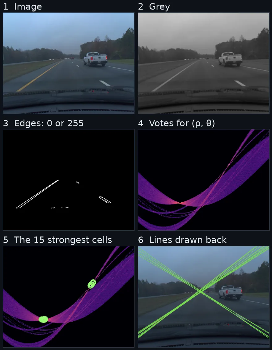
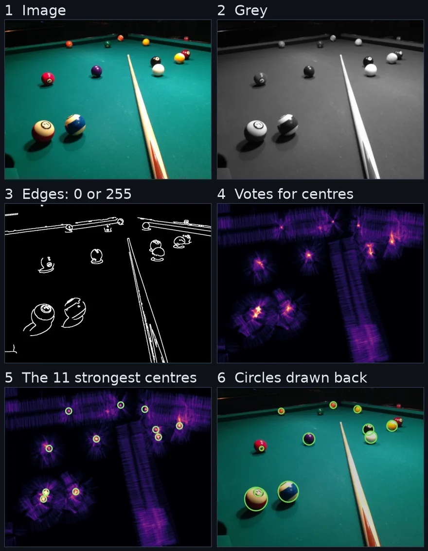
1. Image. A colour photo: three numbers per pixel.
2. Grey. One brightness number per pixel. The outline of a lane marking or a ball is where the brightness changes, and that survives without colour.
3. Edges, as 0 or 255. Every pixel becomes black or white: white where it may sit on the boundary of something. Here the white pixels come from the Canny detector of unit 3.1. A threshold on brightness or colour, cleaned up with morphology, is the other common way to get there. That is unit 2.2, Binary images, not written yet; for now the colour mask and morphology lessons of OpenCV in Practice cover it.
4. Vote. Each white pixel lists every line (or circle) it could belong to and gives each of them one vote. To keep the count, each possible line needs a name made of a few numbers, which is what the two sections after the next one are about.
5. Pick the best. The lines with the most votes are the ones the image contains. A threshold decides how many votes are enough.
6. Use them. Draw them on the image, or read off the numbers: the angle and position of a line, the centre and radius of a circle.

What the numbers are used for

You have met this pipeline in many products, and the numbers it returns are what those products act on:

• Lane-keeping assist. With the two lane lines found, the point where they meet (the vanishing point) slides left or right when the car’s heading turns away from the road’s, and where each line crosses the bottom of the picture says how far the car sits from the middle of its lane. A controller turns the steering wheel to keep both steady. A straight line cannot bend, so for curves the lane is modelled as a parabola, $x = a y^2 + b y + c$, whose $a$ says how sharply the road turns.
• Document scanners. Four lines give the four corners of the page, and the corners give the homography of unit 3.5 that flattens it.
• Court and pitch graphics in sports broadcasts, which start from the painted lines.
• Coin, cell and ball counters. Each circle is a position and a size: how many coins and of which value, where each ball sits on the table.
• Inspection of parts, which checks that a drilled hole is round and an edge is straight.

Lines and circles can be found by letting every edge pixel vote for the shapes it could belong to, and on a real road and a real pool table that finds the lane markings and most of the balls. Every result in this unit is checked against what a person drew by hand: lane markings painted on 300 dashcam frames of the comma10k dataset, and 41 pool balls. On the frame the lessons use, the 15 lines with the most votes all lie on paint; on a typical frame of the dataset only half of them do (median 50%), and two restrictions on the vote take that to 100% on the frames that keep a line (108 of 299 keep none). Fitting a line to one lane dash gives answers 5.1° apart depending on how the distance to the line is measured. Hough circles find 27 of 41 balls with one false circle, close to the 29 a colour pipeline finds.

Before this

You need Edge detection, unit 3.1: every lesson here starts from a Canny edge map, and lessons 2 and 4 vote along the edge direction from image gradients. Lesson 3 meets the same least-squares problem as RANSAC.

How to write down a line

To vote for lines, every possible line needs a name made of a few numbers, and the box that holds the votes, one cell per name, has to be finite.

The form from school is $y = mx + b$: $m$ is how steep the line is (how much $y$ changes when $x$ moves one pixel) and $b$ is where it crosses $x = 0$. In image coordinates, with $x$ to the right, $y$ down and the origin in the top-left corner, the lane line left of the car in the highway frame is

$$y = -0.65\,x + 755$$

That works for this line and fails for steep ones. A lane marking straight ahead of the car, as during a lane change, is close to vertical in the picture, and the slope of a line grows without limit as it turns toward vertical:

angle from horizontal	size of the slope $m$
33° (the left lane)	0.65
45°	1
80°	5.7
89°	57.3
90° (vertical)	none

A vertical line, $x = 600$, has no $m$ and no $b$ at all. A box of votes over $m$ would need cells from minus infinity to infinity, and the cells it can have are badly spread: going from $m = 1$ to $m = 2$ turns the line by 18.4°, while going from $m = 50$ to $m = 51$ turns it by 0.02°.

The fix describes a line by the shortest path from the origin to it: the length of that path, $\rho$, and its direction, $\theta$. Every pixel $(x, y)$ on the line satisfies

$$\rho = x \cos\theta + y \sin\theta$$

The left lane line is $(\rho, \theta) = (633, 57°)$, the vertical line $x = 600$ is $(600, 0°)$, and the horizontal line $y = 500$ is $(500, 90°)$. Every line in the picture has a name with $\theta$ between 0° and 180° and $\rho$ no longer than the image’s diagonal, 1,456 px for this frame, so the box of votes is finite: with 1° and 1 px cells, OpenCV’s layout has 733,860 of them. Duda and Hart made this change in 1972, because with slope and intercept “both the slope and the intercept are unbounded” [3].

For one pixel, sweeping $\theta$ from 0° to 180° traces every line through it as a curve in the $(\rho, \theta)$ box: the purple curves of step 4 above. Lesson 1 works this out on three pixels of the lane line.

How to write down a circle

A circle is every point at distance $r$ from a centre $(a, b)$:

$$(x - a)^2 + (y - b)^2 = r^2$$

The biggest ball on the close-up pool photo is the circle $(a, b, r) = (179, 504, 52)$. Every circle in the picture has a name of this form, with three numbers instead of two, and the third number is what makes it expensive. The box of votes has a cell for every centre at every radius, which on a 960×720 photo searched from 8 to 60 px is 36,633,600 cells, and every edge pixel votes for a whole cone of them. The edge direction cuts that down: on a circle’s outline it points at the centre, so each pixel needs only two votes per radius. Lesson 4 builds it.

Topics

1. The Hough transform. One pixel is one curve of possible lines; a line is where many curves cross. The vote built from scratch, then checked against cv2.HoughLines [3].
2. The probabilistic Hough transform. On a real road the full vote reports lines that are not lanes. Voting only near each pixel’s edge direction [1], dropping lines no lane can follow, and returning segments with two ends [4] is what makes it usable.
3. From segments to the lane: fitting a line. The vote returns several short segments per marking; the car needs one line per side with a precise angle. Least squares, why its answer changes with the axis it treats as the error, and the fit that measures distance at right angles [1].
4. The Hough circle transform. The same vote with three numbers, on the pool table: one radius at a time, then through cv2.HoughCircles [5].

The order follows the pipeline. Lesson 1 is the vote itself, lesson 2 where it breaks on real roads and the fix, lesson 3 the last step from what the vote returns to the numbers a car uses, and lesson 4 the same vote for a shape with one more number.

The two scenes

Lines: a highway. Lessons 1 to 3 work on frame 0825 of comma10k [6], a dashcam photograph of a two-lane highway from a car’s windscreen, 1164×874. Its point is the second image that comes with it: a mask in which volunteers painted every lane marking by hand. Every line the lessons find is scored against that paint, and the same scoring runs on 299 other frames of the dataset, from many cars, roads and times of day.

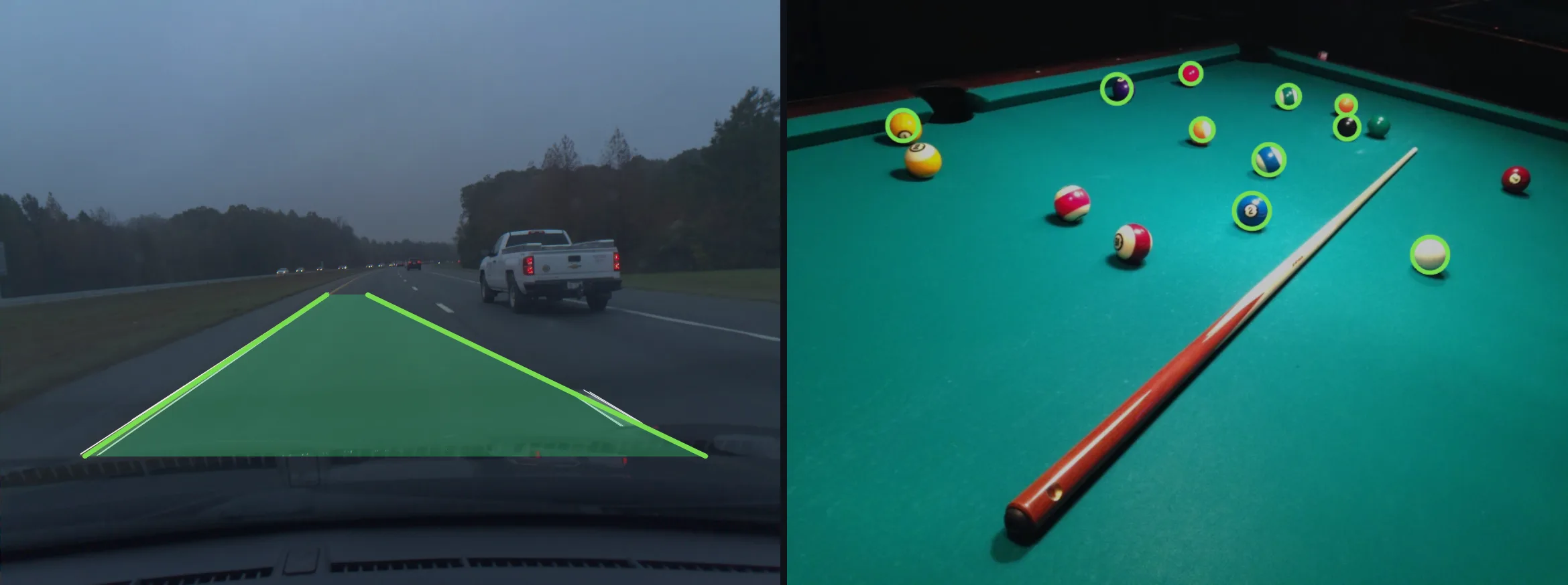
Circles: a pool table. Lesson 4 works on the three pool photographs of OpenCV in Practice M2, where every one of the 41 balls on the cloth was labelled by hand with its centre and radius. That module found 29 of them by colour; lesson 4 finds them by shape and compares. A ball is a sphere, so it looks round from any angle, which is what makes the circle model the right one here.

Two scenes instead of one is a deliberate exception to how this track works: a lane line has no circle in it and a pool table has no long straight line worth fitting, and inventing a picture that held both would leave nothing to score against.

What the unit measures

Every number below is a key in output/boundary_numbers.json.

Result	Measurement
One lane line becomes a fan of lines	On the clean frame, all 15 lines over 60 votes lie on paint, but on only 2 painted lines: 10 on one, 5 on the other
On a typical frame, half the lines are not lanes	Over 299 frames the full vote’s lines are a median 50% on paint
Restricting the vote removes them, at a price	Dropping near-horizontal lines and voting within ±5° of the gradient: median precision 100%, but 108 of 299 frames keep no line at all (92 with the angle restriction alone)
The accumulator is the one OpenCV runs	The from-scratch accumulator returns cv2.HoughLines’ 15 lines with the same votes
Least squares depends on which axis it treats as the error	On one lane dash, y on x gives 28.42° and x on y 33.52°; total least squares 29.67°. Over 473 lane markings on 299 other frames, the two least-squares lines differ by more than 1° on 33%. Turned to near vertical, the dash’s y-on-x line is off by 81° (8.22° against 89.67°)
Hough circles against hand labels	HOUGH_GRADIENT_ALT finds 27 of 41 balls with 1 false circle, median radius error 1.3 px; colour and contours found 29 with 2

Limitations & caveats

• The scoring has a tolerance. A line counts as “on paint” when at least half of its edge pixels lie within 3 px of a painted marking. A wider tolerance would score more lines as correct; the number is a choice, stated in every table.
• The masks are volunteer paint. comma10k’s labels were drawn by the public and reviewed by the project. They are good enough to score against and not a survey: a marking painted a pixel too wide or a faded dash left out moves the scores a little.
• The 299 frames are a sample, not the dataset. Every 33rd file of the 9,888, 57 of them bright enough to call daytime by mean grey level. They are many cars and roads, and they are not a benchmark.
• 41 balls is small. Three photos of one table under one light. The param2 that works there was chosen on one photo and scored on the other two, which is an honest test and a small one.
• Steering and curvature are not measured here. The uses listed above are what these numbers feed in real systems; this unit stops at the lines and builds no controller and no curve fit.
• Nothing is timed. Vote counts are deterministic and make the cost argument on their own.

What this means for your pipeline

• Finding lane lines with Hough: look only at the road, restrict the angles a lane can take, and vote along the gradient. Each step raises precision and lowers how often anything is found; on these frames the last step takes the frames with no line from 92 to 108 of 299.
• Turning segments into one line: use total least squares (cv2.fitLine with DIST_L2). Least squares $y = mx + b$ fails near vertical for the same reason the vote cannot use it, and $x = my + b$ fails near horizontal, by up to 81° on one dash turned the wrong way.
• Counting round things: HoughCircles works without colour and comes within two balls of a colour pipeline here, with fewer false circles. It misses small far balls and green balls on green cloth, and it finds printed circles on the balls themselves.
• What this does not tell you: curved lanes, rain and glare at night, or a table seen from overhead with balls in a rack. The 299 frames include some of each and nothing is tuned for them.

Your turn: other shapes

Any shape with a few unknown numbers can be found the same way. For each one below, write down its equation, count the unknowns, and work out how big the box of votes would be and what one edge pixel votes for.

1. A curved lane, $x = a y^2 + b y + c$.
2. A square of any size, anywhere, turned at any angle.
3. An ellipse, the shape a round coin takes when the camera looks at it from the side.

Answers

1. The parabola has three unknowns, $a$, $b$ and $c$, so the box is three-dimensional, like the circle’s: with 100 values each, a million cells. For a chosen $a$ and $b$, one edge pixel fixes $c$, so each pixel votes along a whole surface of the box. The edge direction gives the slope of the curve at that pixel, $dx/dy = 2ay + b$, which fixes $b$ once $a$ is chosen and leaves one vote per value of $a$: the same trick that turns the circle’s cone into two votes per radius.
2. The square needs its centre $(x, y)$, its side $s$ and its rotation $\varphi$: four unknowns. On a 960×720 photo with 50 sizes and 90 angles that is 3.1 billion cells, which is why nobody votes for squares directly. The practical route is the line vote of lessons 1 and 2, then looking for four lines that meet at right angles.
3. The ellipse needs its centre, its two axes and its rotation: five unknowns. For shapes with no short equation at all, Ballard generalised the transform to arbitrary shapes in 1981 [9].

Where this lands

Lesson 2’s segments are what a document scanner straightens with the homography from unit 3.5, and the classic lane pipeline continues from lesson 3’s lines to fitting a curve per lane. The unit has no measured closer yet; under the track’s rule it ships as a fundamentals lecture and links one when it exists.

How these numbers were made

Parameter	Value
CPU	12th Gen Intel Core i7-12700H, 20 threads
GPU	none used; every step here runs on the CPU
RAM / OS	31 GB · Ubuntu 22.04.5 LTS, kernel 6.8.0-138
Key versions	Python 3.12.9, OpenCV 5.0.0, NumPy 2.5.2. The page’s cells run OpenCV 4.11.0 [7] in Pyodide 314.0.7 and reproduce every number they print
Data (lines)	comma10k [6], imgs/0825_e61068239ce72500_2018-11-13--21-06-53_13_903.png and its mask, MIT; served losslessly at /blog/boundary-detection/highway.webp. Held out: every 33rd file of the listing, 299 frames
Data (animation)	comma2k19 [8], segment b0c9d2329ad1606b|2018-08-03--10-35-16/13, MIT
Data (circles)	The three CC0 pool photos of OpenCV in Practice M2 at 960 px, as the site serves them, and its 41 hand labels
Data (in the wild)	“The Cloister Mandapam, in One point perspective” by Sindugab (lessons 1, 3) and “Stationery on a bench” by Brigitte Tohm via Unsplash (lesson 2), both Wikimedia Commons, CC0; 100 frames of VisA candle (Zou et al., ECCV 2022, Amazon, CC BY 4.0) for lesson 4
Pipeline	road trapezoid at (2%, 78%), (42%, 50%), (58%, 50%), (98%, 78%) of the frame; Gaussian σ 1.4; Canny 25 and 75; Hough at 1 px, 1°, threshold 60
Scoring	a line or segment is on paint when half of its pixels lie within 3 px of the mask; a circle finds a ball when its centre is within the ball’s radius (8 px minimum), one circle per ball
Commands	uv run boundary-download, then uv run boundary-experiments, boundary-figures and boundary-media
Runs	every number is deterministic: one run. HoughLinesP was run twice and returned identical segments
Excluded	no timing is reported in this unit

Further reading

• Go deeper: Szeliski, §7.4 “Lines and vanishing points” [1], and Gonzalez & Woods §10.2 for the textbook account next to Canny [2].
• The original method: Duda and Hart’s 1972 paper [3] is five pages, explains why (ρ, θ) replaced slope and intercept, and already does circles.
• Related on CondadosAI: Edge detection is the prerequisite · Find every ball on a pool table is the colour answer to lesson 4’s question · What is a homography? is what you do with four lines once you have them.

References

[1] Szeliski, R. (2022). Computer Vision: Algorithms and Applications (2nd ed.), §7.4 “Lines and vanishing points”, §7.4.2 “Hough transforms”, p. 477, and §A.2.1 “Total least squares”, p. 929. Springer. Free PDF

[2] Gonzalez, R. C., & Woods, R. E. (2018). Digital Image Processing (4th ed.), ch. 10, §10.2 “Point, Line, and Edge Detection”, pp. 763–804, including Global Processing Using the Hough Transform, p. 799. Pearson.

[3] Duda, R. O., & Hart, P. E. (1972). Use of the Hough Transformation to Detect Lines and Curves in Pictures. Communications of the ACM, 15(1), 11–15. doi:10.1145/361237.361242. Quoted from the 1971 SRI Technical Note 36 version of the paper.

[4] Matas, J., Galambos, C., & Kittler, J. (1998). Progressive Probabilistic Hough Transform. Proceedings of the British Machine Vision Conference 1998. doi:10.5244/C.12.26

[5] OpenCV 4.11.0 source, modules/imgproc/src/hough.cpp (HoughCircles), commit 1d3b34d.

[6] comma.ai (2020). comma10k: 10k crowdsourced images for training segnets. MIT licence. github.com/commaai/comma10k

[7] OpenCV 4.11.0 source, modules/imgproc/src/hough.cpp (HoughLines, HoughLinesProbabilistic), commit 1d3b34d.

[8] Schäfer, H., Santana, E., Haden, A., & Biasini, R. (2018). A Commute in Data: The comma2k19 Dataset. arXiv:1812.05752. MIT licence.

[9] Ballard, D. H. (1981). Generalizing the Hough transform to detect arbitrary shapes. Pattern Recognition, 13(2), 111–122. doi:10.1016/0031-3203(81)90009-1