
Before this unit: Edge detection
What Is the Hough Transform? Finding Lines by Voting
The Hough transform finds straight lines by letting every edge pixel vote for every line that could pass through it. On a dashcam highway frame, 1,749 edge pixels cast 314,820 votes and the 15 strongest lines all lie on painted lane markings, but on only two of them. A from-scratch accumulator matches cv2.HoughLines vote for vote.


The Hough transform finds straight lines by letting every edge pixel vote for every line that could pass through it, and keeping the lines that collect the most votes. Below, the car’s lane found that way on seven seconds of freeway.
You have met it in:
- Classic lane detection in driver-assistance pipelines, as in the animation.
- Document and receipt scanners, which find the page’s sides and its tilt.
- Sudoku and chessboard readers, which find the grid before reading the cells.
- Photo straightening tools, which find the dominant lines of a building and level them.
cv2.HoughLines, the OpenCV call this lesson rebuilds.
Nobody tells the Hough transform which pixels belong together: every edge pixel votes for
every line it could lie on, and the lines with the most votes win. On a dashcam frame, the
15 lines with more than 60 votes all lie on painted lane markings, but on only 2 of
them: one marking comes back as a fan of ten lines. The version built here from scratch matches
cv2.HoughLines vote for vote.
Where we are
Lesson 1 of Boundary detection, and steps 4 and 5 of the unit’s pipeline: the vote, and picking the lines with the most votes. The input is step 3, a black and white edge map from Canny. A frame has thousands of edge pixels, from lanes, cars, shadows and the car’s own hood, and none of them is labelled with the line it belongs to. The vote needs no such grouping, which is why Gonzalez and Woods call it global processing [5].
Naming a line
To count votes for lines, each line needs a name made of a few numbers, and there must be a finite number of names. The form from school, , fails the second test. The slope grows without limit as a line turns toward vertical (57.3 at 89°) and a vertical line has no slope at all, yet a lane marking straight ahead of a car is close to vertical in the picture. Hough’s 1962 patent used slope and intercept [3]; Duda and Hart replaced them in 1972 because “both the slope and the intercept are unbounded” [2].
Their form names a line by the shortest path from the origin to it: its length and its direction . In image coordinates, with the origin in the top-left corner, to the right and down, a pixel lies on the line if and only if
With in and no larger than the image diagonal, every line in the picture has a name and there are finitely many: at 1° and 1 px per cell, OpenCV’s layout for this 1164×874 frame has 733,860 cells. The unit hub works the same comparison on the highway’s own lane line.
One point, every line through it
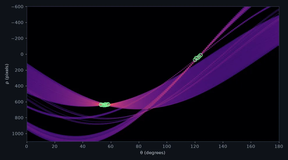
Through a single pixel pass infinitely many lines, one for every angle. For a fixed pixel, as sweeps from 0° to 180°, traces a sinusoid, and every point of that curve is a line through the pixel. Pixels on one common line have curves that all pass through the same , so the line is where the curves cross. Chop the plane into cells, let every pixel add one vote to each cell its curve crosses, and lines become the cells with the most votes [1].
Now you try
Click the frame to add pixels and watch each one become a curve; the busiest cell is drawn back as a line. Start from the worked example’s three pixels.
Then let every edge pixel on the road vote. The threshold sets how many votes a cell needs to count as a line; the bin sets how wide a cell is.
How close is this to OpenCV?
The accumulator is a few lines of NumPy, and cv2.HoughLinesWithAccumulator returns OpenCV’s
lines with their votes, so the two can be compared cell by cell on the highway frame (comma10k,
MIT [6]). The edges are kept only inside a fixed trapezoid over the road ahead: trees,
guard rails, bridges and the car’s own hood are full of straight edges that are not lane lines.
import numpy as np
import cv2

img = cv2.imread("highway.webp")
h, w = img.shape[:2]
gray = cv2.cvtColor(img, cv2.COLOR_BGR2GRAY)
blur = cv2.GaussianBlur(gray, (0, 0), 1.4)

# only the road ahead: a fixed trapezoid
road = np.zeros((h, w), np.uint8)
corners = [(0.02, 0.78), (0.42, 0.50),
           (0.58, 0.50), (0.98, 0.78)]
poly = np.array([(fx * w, fy * h)
                 for fx, fy in corners], np.int32)
cv2.fillPoly(road, [poly], 255)
edges = cv2.Canny(blur, 25, 75) & road

ys, xs = np.nonzero(edges)
xs = xs.astype(np.float32)
ys = ys.astype(np.float32)
n_rho = 2 * (w + h) + 1
half = (n_rho - 1) // 2

acc = np.zeros((n_rho, 180), np.int32)
ang = np.float32(0)
step = np.float32(np.pi / 180)
for t in range(180):
    c = np.float32(np.cos(np.float64(ang)))
    s = np.float32(np.sin(np.float64(ang)))
    r = np.rint(xs * c + ys * s).astype(int)
    acc[:, t] = np.bincount(r + half, minlength=n_rho)
    ang = np.float32(ang + step)

print(len(xs), "edge pixels,", len(xs) * 180, "votes")
r, t = np.unravel_index(acc.argmax(), acc.shape)
print("strongest:", acc.max(), "votes at rho",
r - half, "theta", t)1749 edge pixels, 314820 votes strongest: 362 votes at rho 633 theta 57
# OpenCV's rule for a line: over the threshold, and a
# local maximum against its four neighbours
A = np.pad(acc, 1)
m = A[1:-1, 1:-1]
peak = ((m > 60) & (m > A[:-2, 1:-1])
        & (m >= A[2:, 1:-1]) & (m > A[1:-1, :-2])
        & (m >= A[1:-1, 2:]))
ours = set(zip(*np.nonzero(peak)))

ref = cv2.HoughLinesWithAccumulator(
    edges, 1, np.pi / 180, 60).reshape(-1, 3)
cv = {(round(rr) + half, round(np.degrees(tt)))
      for rr, tt, _ in ref}
print("ours:", len(ours), " OpenCV:", len(cv))
print("same lines:", ours == cv)
print("same votes:", all(
    acc[round(rr) + half, round(np.degrees(tt))] == v
for rr, tt, v in ref))ours: 15 OpenCV: 15 same lines: True same votes: True
The two agree on all 15 lines and every vote, with two details copied from OpenCV’s source [4]: is computed in 32-bit floats, and the angle table is built by adding the step to a 32-bit angle 180 times. On this frame the same accumulator in 64-bit floats from exact angles also agrees; on other images it can put a vote one cell over whenever a lands within a rounding error of half a pixel, which is worth knowing the next time two Hough implementations disagree by a line.
In the wild
The same accumulator on a cloister photographed in one-point perspective, where every receding line points at one vanishing point, as the lane lines of a straight road do [1]. Its 12 strongest oblique lines are intersected in pairs; the 32 pairs within about 12° of parallel are skipped, because two nearly parallel lines cross at a poorly defined point:
| lines over 80 votes | 2,771 |
| pair intersections used | 34 |
| within 20 px of their median point | 94.1% |
| median distance to that point | 5.3 px |
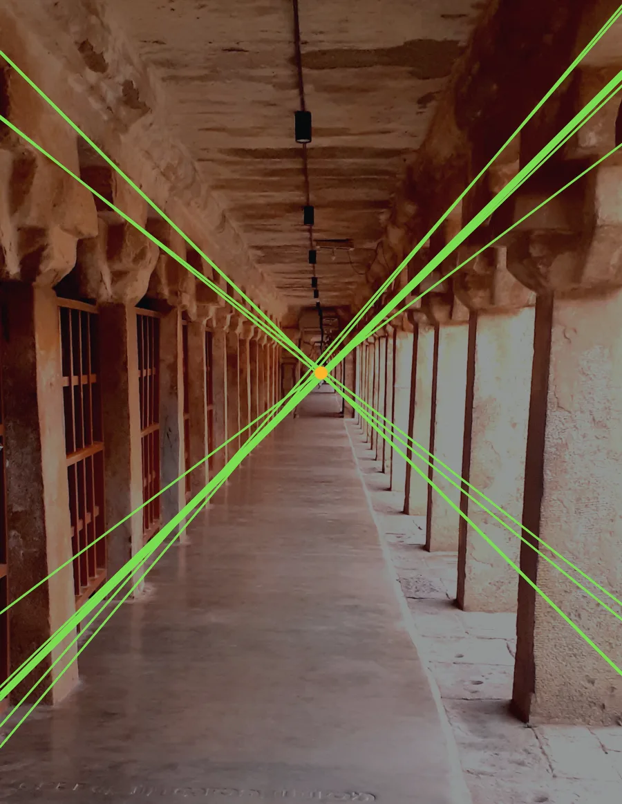
What it means: the strongest peaks are real lines, accurate enough that their crossings agree to a few pixels. The 2,771 lines over the threshold are the other half: a richly textured photograph spreads votes everywhere, and a threshold alone cannot separate a corridor from its floor tiles.
Where this breaks
One lane line becomes a fan of lines. All 15 lines over 60 votes lie on paint, but 10 sit on the solid line left of the car and 5 on the dashed one to the right. The cells next to the strongest one, (641, 55°) with 309 votes, (635, 58°) with 140, (637, 54°) with 122, are the same painted line: a marking is several pixels wide and slightly curved, so its votes spill into neighbouring cells, and every spill that is a local maximum somewhere is reported.
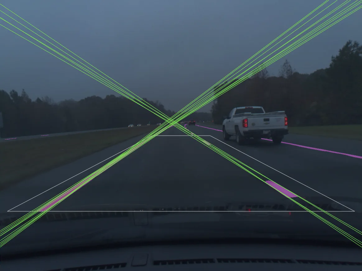
The threshold and the bin size move the answer.
| threshold (1° bins) | lines | on paint | paint covered |
|---|---|---|---|
| 40 | 33 | 33 | 98.3% |
| 60 | 15 | 15 | 89.4% |
| 120 | 4 | 4 | 61.8% |
| 200 | 2 | 2 | 58.6% |
At 0.5° bins and a threshold of 60 the count is 31; at 2° it is 10. There is no setting at which two painted lines give two lines.
On a typical frame, half the lines are not lanes. The frame above is clean. Over 299 other comma10k frames, with the same trapezoid and thresholds, the full vote returns a median of 17 lines of which a median 50% lie on paint, and on 42 frames it finds nothing. The rest come from guard rails, car outlines, shadows, a hood that reaches into the trapezoid on some cars, and road texture.
The cost is every pixel times every angle. 314,820 votes for one frame, almost all of them for lines that do not exist.
All four come from the same choice: every pixel votes at every angle, although image gradients already measured which way its edge runs, and although no lane line seen from a car runs flat.
Exercises
- Find the shared cell. Using the three pixels of the worked example, compute at
every whole degree and return the that all three share as
cell, with rounded to a whole pixel.
pts = [(490, 437), (318, 548), (119, 678)]
cell = (0, 0)  # (rho, theta in degrees)
print(cell)- Predict, then run. Rebuild the accumulator with 0.5° bins (360 columns, step
np.pi / 360) and count the lines over 60. Write down the count and the strongest vote first. - Move the threshold. Count the lines over 40, 120 and 200 votes with the 1° accumulator, and check which painted line each one lies on. Is there a threshold that gives one line per painted line?
What you should see
These come from section 1 of the unit notebook, boundary_detection.ipynb, and are the same on
OpenCV 4.11 (this page) and 5.0.
(633, 57).- 31 lines, all on paint, and still 362 votes at the strongest cell.
- 33, 4 and 2, and no. At 120 and at 200 every line left is on the solid line on the left (the two at 200 have 362 and 309 votes); the dashed line’s best cell has 94 votes, fewer than the solid line’s fifth. A long solid line outvotes a dashed one at every threshold, which is one more reason lane code stops treating the threshold as the answer.
Check yourself
Four questions on this lesson. Pick an answer to see why it is right or wrong.
In the Hough transform, what does one edge pixel become in the (ρ, θ) accumulator?
For a fixed pixel, ρ = x cos θ + y sin θ traces a sinusoid as θ sweeps 0° to 180°. Every cell on it is a line through that pixel, and lines are where many sinusoids cross.
On the highway frame, all 15 lines over 60 votes lie on painted markings. How many markings do they cover?
Ten lines sit on the solid line on the left and five on the dash. Neighbouring cells of one thick, slightly uneven marking all clear the threshold.
With 0.5° bins instead of 1°, at the same threshold of 60, how many lines come out?
Finer bins split one marking over more cells, and more of them clear 60. At 2° bins the count is 10. The answer moves with a setting that has no principled value.
How many votes does the full vote cast on the frame, and why so many?
1,749 edge pixels times 180 angles. Almost every vote lands on a line that is not there, which is what lesson 2 attacks.
Next
Every problem above comes from letting each pixel vote at every angle. Lesson 2 restricts the vote to the angles a pixel’s gradient and a lane allow, and then stops voting for whole lines.
References
[1] Szeliski, R. (2022). Computer Vision: Algorithms and Applications (2nd ed.), §7.4.2 “Hough transforms”, p. 477, and §7.4.3 “Vanishing points”, p. 481. Springer. Free PDF
[2] Duda, R. O., & Hart, P. E. (1972). Use of the Hough Transformation to Detect Lines and Curves in Pictures. Communications of the ACM, 15(1), 11–15. doi:10.1145/361237.361242. Quoted from the 1971 SRI Technical Note 36 version of the paper.
[3] Hough, P. V. C. (1962). Method and means for recognizing complex patterns. US Patent 3,069,654. Google Patents
[4] OpenCV 4.11.0 source, modules/imgproc/src/hough.cpp: createTrigTable (lines 84–93) and findLocalMaximums (96–108), commit 1d3b34d.
[5] Gonzalez, R. C., & Woods, R. E. (2018). Digital Image Processing (4th ed.), ch. 10, §10.2 “Point, Line, and Edge Detection”, Global Processing Using the Hough Transform, p. 799. Pearson.
[6] comma.ai (2020). comma10k: 10k crowdsourced images for training segnets. MIT licence. github.com/commaai/comma10k