
Before this unit: Edge detection
Fitting a Line to Points: Least Squares vs Total Least Squares
The line you fit to a set of points depends on how you measure the distance to it. Worked by hand on eight pixels of a painted lane dash: least squares y on x gives 18.5°, x on y gives 32.7°, total least squares 20.2°. Over 473 lane markings, the two least-squares lines differ by more than 1° on a third of them.
Line fitting finds the one straight line that passes closest to a set of points. Below, the car’s lane found on seven seconds of freeway: each green boundary is one line fitted to the lane-marking pixels on that side of the car.

You have met it in:
- Trend lines in a spreadsheet, which are least squares y on x, the first fit here.
- Lane-detection pipelines, which usually fit x as a function of y, the second fit here.
- Straightness checks in machine vision, which fit a line to an edge and report how far the pixels stray from it.
cv2.fitLine, OpenCV’s line fitter, which is the third fit here.
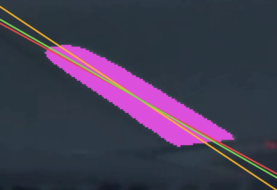
The best line through a set of points depends on how you measure each point’s distance to it, and the usual shortcut gives a different line depending on which way the picture is turned. On the 1,955 painted pixels of one lane dash, least squares with y as a function of x gives a line at 28.42°, with x as a function of y 33.52°, and total least squares, which measures distance at right angles, 29.67°. Stand the dash upright and y on x is off by 81° while total least squares follows it. Over 473 lane markings on 299 other dashcam frames, the two least-squares lines differ by more than 1° on a third of them.
Where we are
Lesson 3 of Boundary detection, and the last step of its pipeline. Lesson 1 voted for lines and lesson 2 cleaned the vote up and returned segments. What comes out is several short segments per lane marking, each with a direction read off a 1° cell. A car steers by one line per side with a precise angle, and getting it means fitting a line through the pixels the vote grouped together; Gonzalez and Woods treat that step in the same section as Canny [2].
The question for this lesson is only which line is the best through a set of pixels that belong together. To compare the fits on pixels known to be on a marking, it uses the pixels of one dash painted by comma10k’s labellers [3] rather than the vote’s segments.
Three ways to measure “closest”
A line is closest to a set of points when the distances from the points to it are small, squared and summed. The choice is which distance.
Least squares, y on x, writes the line as and measures each point’s distance vertically. With the points centred on their mean , the best slope is
Least squares, x on y, swaps the roles: , horizontal distances, . Lane-detection code usually does this, because lanes seen from a car are steep.
Total least squares measures each point’s distance at right angles to the line, the distance anyone would draw with a ruler. The best line passes through the mean along the direction in which the points spread most, the first principal direction of the matrix of centred sums [1]:
The first fit ignores and the second ignores . Only the third uses all three sums, which is why it is the only one that gives the same line however the picture is turned.
Now you try
The eight pixels from the worked example. Cycle through the three kinds of residual, then rotate the points and watch which least-squares line runs off first.
How close is this to OpenCV?
All three fits take a few lines of NumPy, and cv2.fitLine with DIST_L2 is OpenCV’s total
least squares. The cells load the dash’s painted pixels from the frame’s mask and fit them three ways.
import numpy as np
import cv2

# the dash's pixels, painted by comma10k's labellers
mask = cv2.imread("dash-mask.webp", cv2.IMREAD_GRAYSCALE)
ys, xs = np.nonzero(mask)
P = np.c_[xs, ys].astype(float)

# least squares, y on x and x on y
m = np.polyfit(P[:, 0], P[:, 1], 1)[0]
m2 = np.polyfit(P[:, 1], P[:, 0], 1)[0]
y_on_x = np.degrees(np.arctan(m)) % 180
x_on_y = np.degrees(np.arctan2(1, m2)) % 180

# total least squares: first principal direction
d = np.linalg.svd(P - P.mean(axis=0))[2][0]
tls = np.degrees(np.arctan2(d[1], d[0])) % 180

print(len(P), "pixels")
print(f"y on x: {y_on_x:.2f}   x on y: {x_on_y:.2f}")
print(f"total least squares: {tls:.2f}")1955 pixels y on x: 28.42 x on y: 33.52 total least squares: 29.67
v = cv2.fitLine(P.astype(np.float32), cv2.DIST_L2,
                0, 0.01, 0.01).ravel()
fit = np.degrees(np.arctan2(v[1], v[0])) % 180
print(f"cv2.fitLine:        {fit:.2f}")
print(f"difference to ours: {abs(fit - tls):.4f}")cv2.fitLine: 29.67 difference to ours: 0.0000
cv2.fitLine agrees with the SVD to four decimal places. It returns a direction and a point on
the line, never a slope, which is the representation that has no trouble with any angle.
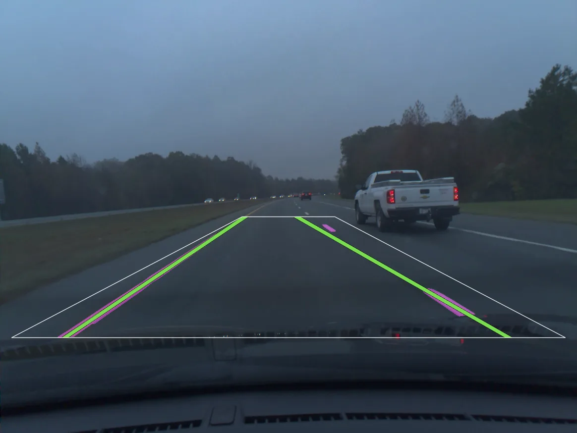
Fitted the same way to each of the frame’s two painted markings, total least squares gives the lane lines: 29.67° for the dash on the right and 146.13° for the solid line on the left. Those two angles, and where the two lines meet, are what a lane-keeping system reads its heading from, as the unit hub describes.
In the wild
A photograph of a temple cloister has a different kind of edge: thin, long and mostly vertical, the columns. Unit 3.1 measured them at a median 2.3 px wide. Fitting y on x and total least squares to the pixels of its ten strongest near-vertical edges:
| least squares, y on x | total least squares | |
|---|---|---|
| edges where the two agree within 0.2° | 6 of 10 | |
| median distance from vertical | 2.12° | 1.42° |
| largest distance from vertical | 62.33° | 2.05° |
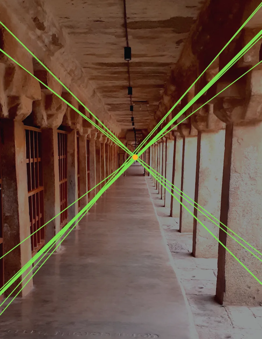
What it means: on a thin edge the fits mostly agree. The two edges where y on x is off by 60° and 62° are the two whose pixels sit in one perfectly vertical column (total least squares returns 90.00° for both): every is the same, is close to zero, and the slope is decided by the few pixels that stray. Lane code fits x on y for this reason.
Where this breaks
Each least-squares fit fails near one axis. Turning the dash’s 1,955 pixels about their centre and refitting:
| turned by | y on x | x on y | total least squares |
|---|---|---|---|
| 0° (as painted) | 28.42° | 33.52° | 29.67° |
| 30° | 55.92° | 60.96° | 59.67° |
| 60° (nearly vertical) | 8.22° | 89.68° | 89.67° |
| 90° | 123.52° | 118.42° | 119.67° |
At 60° the dash stands at 89.67°, and y on x reports 8.22°, wrong by 81°. x on y is right there and is the worse of the two at 0°. Total least squares is right at every angle. On real frames the size of the problem varies with the marking: over 473 markings on 299 frames, the two least-squares lines differ by a median 0.46°, by more than 1° on 33%, and by up to 38°.
None of the three survives a real outlier. All are sums of squares, so a pixel far from the line carries the square of its distance. On the dash’s 1,955 pixels one stray pixel barely moves anything; a car’s edge, a crack or the next dash is hundreds. The answer for outliers is to stop squaring them, which is what RANSAC does.
All three trust the grouping. The dash was picked out by a person’s paint on a mask. In the lane pipeline the grouping comes from the vote of lessons 1 and 2, and a segment it puts on the wrong side, from a guard rail or a car, enters the fit as an outlier with its whole length.
Exercises
- Total least squares by hand. Write
tls_angle(P), the angle in of the total least squares line through an array of points, from the centred sums and the formula above (no SVD, no OpenCV). It must matchcv2.fitLineon the dash to 0.01°.
def tls_angle(P):
    # centred sums, then the formula
    return 0.0

print(tls_angle(P), fit)- Predict, then run. Turn the dash’s pixels by 60° about their mean
(
R = cv2.getRotationMatrix2D(tuple(P.mean(axis=0)), -60, 1), thenP @ R[:, :2].T + R[:, 2]) and refit all three. Before running, say which least-squares fit will be wrong. - Long and thin against short and wide. Load
line-mask.webp, the painted pixels of the solid yellow line on the left of the frame (5,761 of them), and fit it all three ways. How far apart are the three lines now?
What you should see
These come from section 3 of the unit notebook, boundary_detection.ipynb, and are the same on
OpenCV 4.11 (this page) and 5.0.
- 29.67°, the same as
cv2.fitLine. - The dash now stands at 89.67°. y on x reports 8.22°, wrong by 81°; x on y gives 89.68°.
- 146.19°, 146.02° and 146.13°: within 0.17° of each other. The line is about 450 px long and a few pixels wide, so the spread along it dominates every sum and the choice of axis stops mattering. The dash is about 120 px long and up to 40 px wide.
Check yourself
Four questions on this lesson. Pick an answer to see why it is right or wrong.
Least squares fits y = mx + b. Which distance from each point to the line does it minimise?
Least squares measures the error in y only. That is why a steep marking, where the error is mostly sideways, pulls its line toward horizontal.
The lane dash is turned until it stands at 89.67°, nearly vertical. What does least squares y on x report for it?
With the points stacked almost vertically, the spread in x is tiny and the fit tilts the line to shrink vertical gaps. Total least squares follows the dash to 89.67°.
Over 473 lane markings on 299 frames, how often do y on x and x on y differ by more than 1°?
The median difference is 0.46°, but 33% differ by more than 1° and the worst by 38°. Which way you measure the error is a real choice, not a detail.
Which of the three fits does cv2.fitLine with DIST_L2 compute?
cv2.fitLine with DIST_L2 measures distance at right angles to the line, which is total least squares; it agrees with the SVD on the dash to four decimal places. None of the three survives a real outlier.
Next
Lines are now found, cleaned up and fitted, one per side of the car. A ball, a coin or a wheel is not a line. Lesson 4 votes for circles, with three numbers instead of two, on a pool table where every ball was labelled by hand.
References
[1] Szeliski, R. (2022). Computer Vision: Algorithms and Applications (2nd ed.), §A.2 “Linear least squares”, §A.2.1 “Total least squares”, p. 929. Springer. Free PDF
[2] Gonzalez, R. C., & Woods, R. E. (2018). Digital Image Processing (4th ed.), ch. 10, §10.2 “Point, Line, and Edge Detection”, pp. 763–804. Pearson.
[3] comma.ai (2020). comma10k: 10k crowdsourced images for training segnets. MIT licence. github.com/commaai/comma10k