A Traffic Camera in a Simulated New York: Exact Labels at 0.75 s a Frame

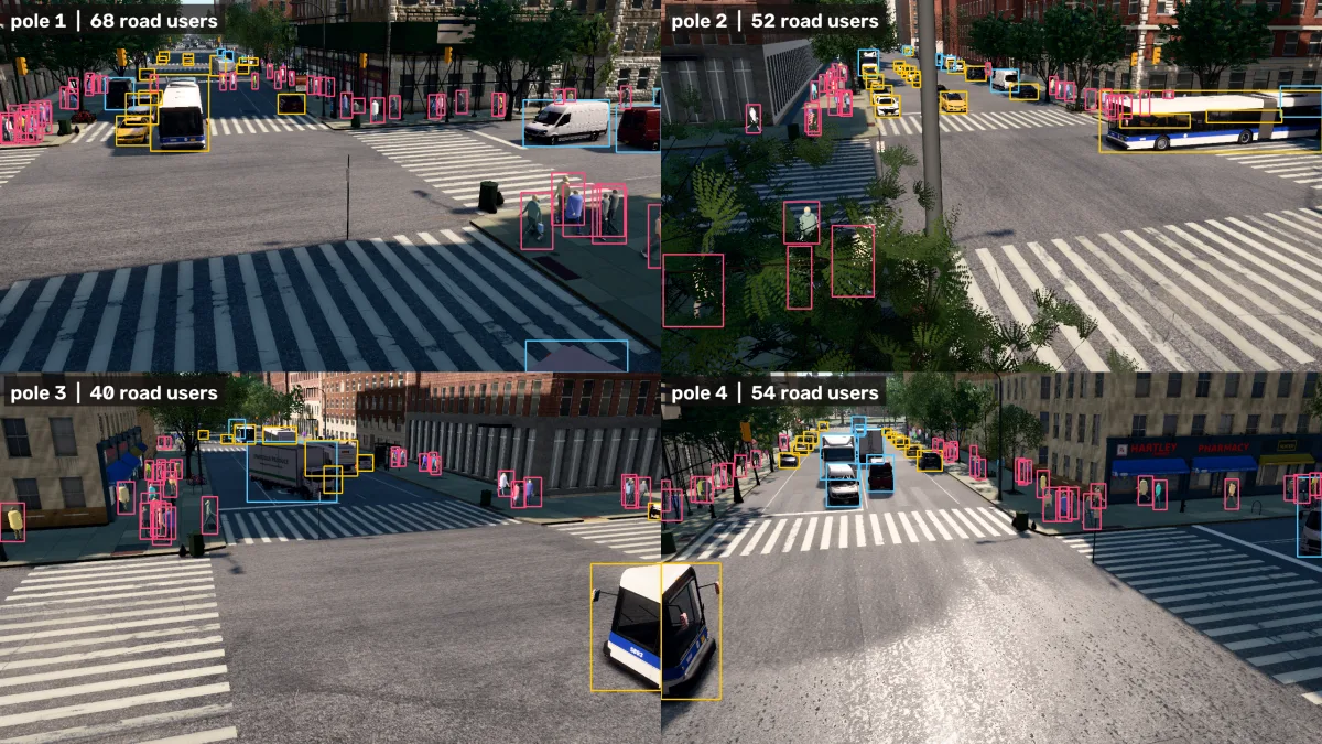
A simulator can stand in for a street camera: it draws a real New York junction, moves cars and people through it, and tells you for every pixel which car or person it belongs to.

Below are twenty seconds from a simulated pole camera at W 120th Street and Amsterdam Avenue in Harlem. The four panels are the same instant: the picture a camera would record, the class of every pixel, a box around every road user, and the distance of every pixel from the lens.

You have met the pieces of this before:

• Traffic cameras that count and classify, the ones on city poles that report how many cars, buses and bikes went through a junction.
• Red-light and speed cameras, which need to know where on the road a vehicle is, as well as that it is in the picture.
• Self-driving simulators such as CARLA [2], where cars learn to drive in a city that exists only as software. Valdrada borrows CARLA’s vehicle models and the shape of its Python API.
• Training data from video games: Richter et al. labelled 24,966 frames of Grand Theft Auto V for segmentation [3], because the game’s renderer already knows what every pixel is.

You can run a simulated New York street camera on one desktop graphics card and get labels nobody has to draw, then record it in a format the same code can later read from a real camera. Four cameras sharing each capture cost 0.75 s per labelled frame on an RTX 5060, so 20,000 frames take about 4.1 hours. The labels are exact in geometry (box, mask, depth and occluded fraction come from the renderer) and only as right as the simulator’s own taxonomy in class: a box truck and a city bus are both labelled car, and night renders as bright as day. A COCO-trained RF-DETR finds 99.5% of the easy vehicles in these frames and 6.4% of the tiny objects.

Szeliski’s advice for testing any vision algorithm starts here: “test your algorithm on clean synthetic data, for which the exact results are known”, then add noise, then go to real data [4, Preface]. A city simulator is that first step at the scale of a street. This post is the first of a series. It covers what it took to get the simulator running and what its labels are; the next one builds a dataset at scale and fine-tunes a detector on it, and the one after builds a traffic-safety system (red lights, near-misses, speed) whose camera can be simulated or real.

The junction and the cameras

Every number here comes from one junction, W 120th St and Amsterdam Ave (the example the Valdrada author ships), and from cameras mounted the way a city would mount them:

	Pole-search camera	Four diagonal poles
Where	14 m north of the junction centre, 8 m up, aimed past the centre	20 m out on each diagonal, 7 m up, tilted 18° down
Chosen by	a search over 48 candidate poses (below)	fixed geometry
Used for	the video above, the recordings, the conditions, the test frames	the cost per frame, the training frames
Road users in view	44 to 48 per frame (six conditions)	54 to 60 per frame on average

Valdrada [1] is an open-source digital twin of New York’s five boroughs, compiled from city records and OpenStreetMap by Mehmet Kerem Turkcan (whose 3D vehicle detector ran on a laptop iGPU here). It renders in a browser engine and is driven from Python like CARLA: spawn a car, spawn a camera, step the world, read the sensors.

What you are about to see, step by step

The picture in the video and its labels come out of one pipeline. The last two steps are what makes the simulated camera replaceable by a real one.

1. Simulated city. The server loads the junction’s map tiles and runs traffic on the street graph. In synchronous mode nothing moves until the script asks for the next step, so a slow camera never misses a frame.
2. Pole camera. A camera is an object placed in the world with a position and an angle, like a real one bolted to a pole.
3. Sensors on the same step. Each output is a separate sensor at the same pose. They all report the same frame number, so the labels belong to the picture they sit next to.
4. Labels. The instance sensor returns, per object, its class, a box around its visible pixels, its pixel area and an id; for the largest objects it also returns the box of the whole object including hidden parts and the fraction hidden (next section) [5].
5. Recording folder. record.py writes the frames, a timestamp per frame and the camera’s intrinsics (the focal length and image centre in pixels, written K) and pose; the labels go to a separate gt/ folder that only an evaluator opens.
6. Any reader. The pipeline gets frames only through a frame source, and a recording folder is one kind of source among a video file, an RTSP stream and a webcam (last section).

Getting it to render on the GPU with no screen

The server is an Electron app: a Chromium browser that draws the city with WebGL. On a machine with no monitor it needs a display to draw into, and if that display has no GPU behind it, Chromium quietly falls back to software rendering. The server reports which renderer it got, and that string is the first thing to check: ANGLE (NVIDIA Corporation, NVIDIA GeForce RTX 5060/PCIe/SSE2, OpenGL 4.5.0) means the GPU, llvmpipe means the CPU is pretending to be one.

I ran it inside a Docker container on a desktop with an RTX 5060 and tried seven combinations of display and graphics backend (ANGLE is the layer Chromium uses to turn WebGL into OpenGL or Vulkan calls). The full table, with each run’s renderer string and benchmark output, is output/render_paths.md in the companion repo. Three of them show the range, from no GPU to the fastest:

Display	Chromium graphics flags	Renderer	Seconds per simulation step, 3 sensors
Xvfb (a virtual screen in memory)	defaults	Mesa llvmpipe, software	the city never finished loading (210 s timeout)
Xvfb	ANGLE over Vulkan	RTX 5060	0.334 to 0.335
headless Xorg on the NVIDIA driver	ANGLE over OpenGL	RTX 5060	0.217 to 0.220

The fastest route runs a real X server inside the container, using the NVIDIA driver’s own X module with no monitor attached (AllowEmptyInitialConfiguration, UseDisplayDevice "None" in the driver’s X configuration [6]), and starts the server with --use-gl=angle --use-angle=gl --ignore-gpu-blocklist. It takes about a third less time per step than Vulkan on Xvfb (0.218 against 0.335 s, the midpoints of two runs each). The Dockerfiles and the X configuration are in the repo.

Valdrada’s own install guide documents a different route for headless Linux: Chromium’s headless platform with ANGLE over Vulkan, tested by the author on an RTX 6000 Ada with no container [7]. In my container, a close variant of it (--ozone-platform=headless plus Vulkan flags) crashed Chromium’s GPU process one second after start. I did not run the documented command as written, and nothing here ran outside the container. This section reports what works in Docker with this driver; the guide’s own route is untested here.

What a simulated label contains

Nobody draws a simulator’s labels, so they have none of the usual slips (a box a few pixels too wide, a missed pedestrian at the back). It has a different kind of error: it is whatever the simulator’s rules say it is. Both matter before anyone trains on it.

The visible box and the whole-object box. Each road user has a box around the pixels you can see (bbox). The largest objects in view (8 per frame here, a setting called amodal) also get the box the object would have if nothing stood in front of it (amodal_bbox, from the term amodal perception: seeing the whole shape of a partly hidden object [5]) and the fraction of it that is hidden:

$$\text{occlusion} = 1 - \frac{\text{visible pixels}}{\text{pixels of the whole object}}$$

Valdrada measures the denominator by rendering the object again on its own [1].

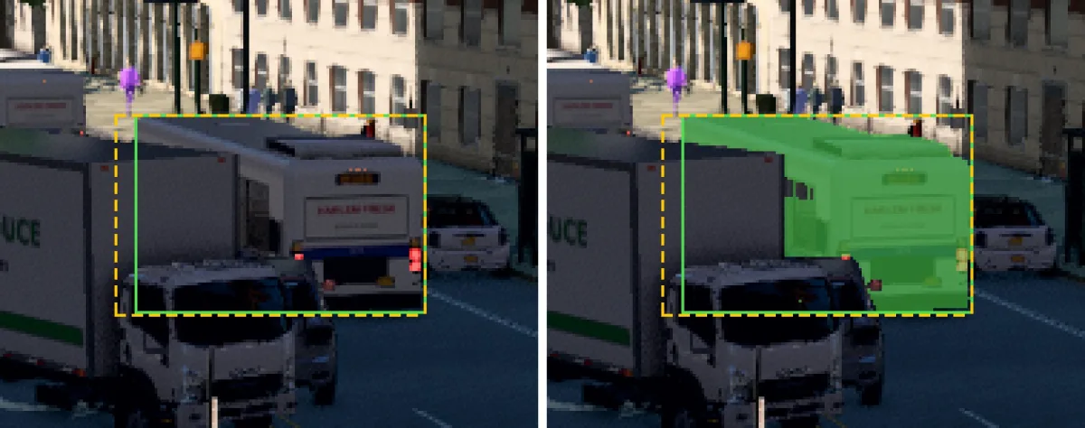
Four more things the labels do that a reader should know before using them:

• The class is the simulator’s. The truck above is car, and so is the articulated bus that all four poles of the cover see, one box per view (poles 3 and 4 both see it up close, so at the bottom its two views meet at the seam). In the 218 frames the detector runs on below, the labels count 3,116 car, 1,432 truck, 6,431 pedestrian and no bus or bicycle; in the other label files I checked (the recordings, the conditions, the second junction), bus appears once, on a 72 px object. A model trained on these labels learns that a bus is a car.
• Most road users have no actor id. In a 100-frame recording, 2,371 of 2,674 road-user labels over 400 px have actor_id 0, the value the static city also gets. Only vehicles created through the API, like the 20 the script spawned, have one; the rest is the server’s own traffic and crowd.
• The instance id is what tracks. Every one of 2,573 boxes that overlap a box in the next frame at IoU above 0.7 keeps its id (2,657 of 2,662 at night). That is identity ground truth for tracking, including for the ambient traffic, and it is what the safety post will score trackers against (the metrics are in the tracking metrics post).
• Small things get labels too. Any object with at least 30 visible pixels (min_pixels, the default) gets a box, so a pedestrian seen through a gap in a tree’s leaves is labelled (pole 2 in the cover). Whether a detector should be expected to find it is a separate question, and the slices further down answer it with the area.

The geometry is exact in the sense that matters for evaluation: the box, the mask, the depth and the occluded fraction are computed from the scene. The camera is exact too: K comes from the field of view, $f = \tfrac{1280/2}{\tan 35^\circ} = 914$ px, the same matrix a calibration would estimate for a real camera.

What a labelled frame costs

The cost that decides whether a dataset is practical is wall-clock seconds per labelled frame. A capture is expensive, and the steps between captures, where the traffic moves on, cost a simulation step each. Cameras that capture on the same step share those in-between steps.

budget.py measured it with one, two and four pole cameras, each producing RGB plus instance labels with 8 whole-object boxes, one capture every 20 steps (1 s of simulated time), 12 captures per setting:

Cameras per capture	Seconds per capture	Seconds per labelled frame	20,000 frames	Road users per frame
1	2.06	2.06	11.4 h	56
2	2.43	1.21	6.7 h	60
4	2.99	0.75	4.1 h	54

The capture itself still grows with each camera (0.23 s for one, 0.81 s for four), so the saving shrinks as cameras are added; I measured only up to four. Pick the camera count and the dataset size and watch the cycle split:

Placing the pole, and what the weather does

A camera placed by coordinates can land inside a tree. Manhattan’s street trees are in the city records, and the simulator places them. check3.py scores 48 candidate poses around the junction (8 directions × 3 distances × 2 heights) on one semantic and one depth frame each, and keeps a pose when under 10% of the frame is vegetation, under 5% is closer than 5 m and over 20% is road. 31 of the 48 pass; of the 17 that fail, 12 fail on vegetation.

At a second junction, Broadway and W 96th St (an eight-arm junction that streamed in 9 to 14 s after the camera moved there, over four runs), I first placed four poles by fixed geometry, 20 m out and 7 m up, and one of them is inside a street tree: 98% of its frame is vegetation and 96% is closer than 5 m. Then I ran the same 48-pose search there (pole_compare.py), and no pose passes. The six on that pole’s corner are all inside trees (74% to 99% of the frame closer than 5 m). Of the other 42, 40 have nothing within 5 m, but Broadway’s tree-lined median puts 11% to 44% vegetation in their frames, over the 10% cap I had set at the first junction; 38 fail on vegetation alone.

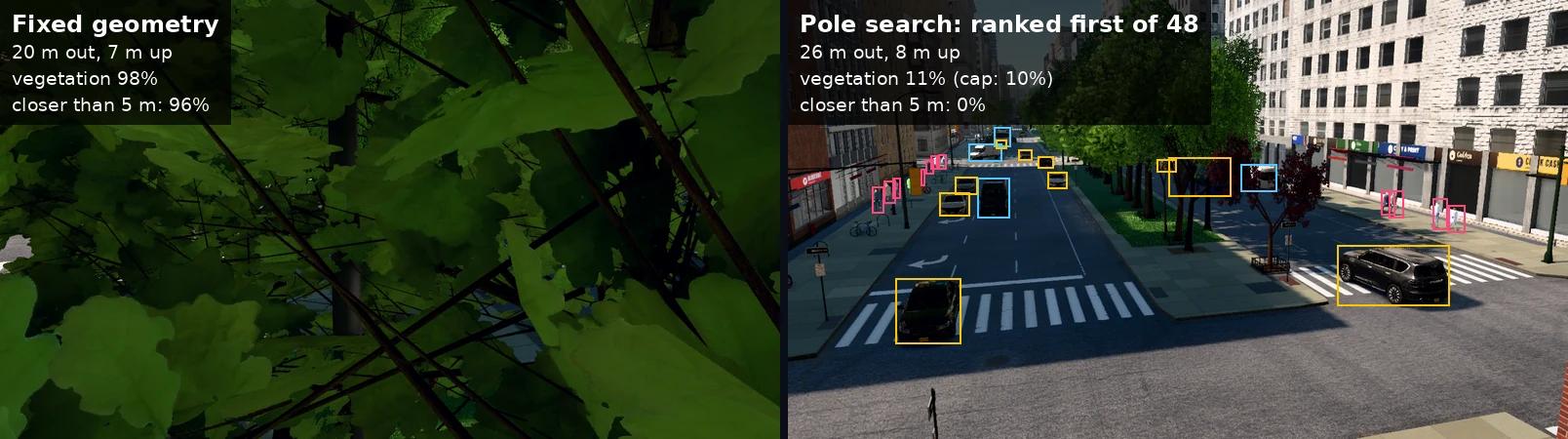
So the test that catches a camera inside a tree is the depth one (96% of the frame within 5 m against 0%). The vegetation share measures how green the street is, and its cap has to be set per junction or dropped.

The pole search also has a blind spot: it rewards road in the frame, and the winning pose at the first junction (14 m out, 8 m up) shows mostly empty asphalt in its lower half, as the video does. It does not yet ask where the road users are; the dataset post will score that too.

Weather and time of day. Valdrada sets the time (day, golden hour, dusk, night) and rain from Python, and the same run can change them between captures:

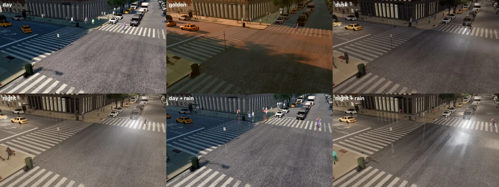
Night here is headlights, lit windows and wet reflections at day brightness: the mean pixel value of the night frame is 107, against 96 by day. The browser renderer adjusts its exposure every frame, like a phone camera. The API has a camera setting, exposure_mode="manual", that the documentation describes as the time of day’s fixed exposure, scoped to RGB cameras “on a renderer client” [8]. I recorded 100 night frames with it and they came out brighter still (mean 110 to 122, against 95 to 97 by day):

Reading the client code, the browser engine keeps its own per-frame meter, and the attribute seems to reach only the packaged Unreal Engine renderer; I did not test that renderer. For a dataset, “night” from this renderer means headlights and a change of colour at normal brightness, and that is what a night slice of an evaluation would test.

How far a COCO detector gets on simulated frames

The question behind a synthetic dataset is whether a model that has seen only real photos recognises the simulated street at all. If it does on the easy cases, the renderer is close enough to real footage to be useful; where it fails is what training on simulated frames has to fix.

RF-DETR Small [9], trained on the 80 everyday classes of the COCO dataset [10] and not adjusted in any way, ran on the 218 labelled frames of the first runs (the cost-per-frame run, the author’s recording script and the site checks). A ground-truth box counts as found when the detector puts a box of a matching class on it with enough overlap. Overlap is measured as IoU, intersection over union: the area the two boxes share divided by the area they cover together, from 0 (apart) to 1 (identical). The threshold here is 0.5, the usual one (the detection metrics post goes through it). Drag the boxes to see where 0.5 falls:

Recall, the share of real road users the detector found, by slice:

Slice	Boxes	Recall
Easy vehicles (under 10% hidden, over 2,000 px, not cut by the frame edge)	443	0.995
Vehicles under 10% hidden	573	0.953
Vehicles 10 to 50% hidden	191	0.806
All vehicles	4,548	0.375
All pedestrians	6,431	0.174
Tiny objects (under 400 px)	6,192	0.064

It also drew 1.1 boxes per frame on road-user classes that matched nothing.

Object detection on real traffic footage fails in the same places, small and far and hidden [4, §6.3 “Object detection”], so this is the ordinary weakness of a COCO model on a pole camera, measured with labels nobody had to draw. The occlusion slices hold only large objects, because only the 8 largest per frame have an occlusion value.

A first fine-tune, as a pipeline check. To see that the labels train a model end to end, I fine-tuned RF-DETR Small on 84 frames from the four diagonal poles (40 epochs, 9 minutes on the RTX 5060), chose the checkpoint on 24 frames from another pose, and scored it on 110 frames from the pole-search camera, a different run of the same junction:

Test slice (110 frames)	Boxes	COCO weights	Fine-tuned
Vehicles 10 to 50% hidden	173	0.832	0.983
All pedestrians	1,834	0.333	0.736
Tiny objects	2,202	0.124	0.374
Unmatched boxes per frame		1.11	3.83

Recall went up everywhere the COCO model was weak, and so did the boxes that matched nothing, from 1.1 to 3.8 per frame. I have not looked into why; some may be objects under the 100 px floor of the ground truth, and the 0.5 confidence threshold was not tuned for either model. Train and test share a junction, so this shows that the labels train a model end to end. What simulated data buys on a new street is the next post’s question, with whole junctions held out.

Record here, run anywhere

The safety system later in this series has to run on a real camera, so it must not know whether its frames come from the simulator. Every frame enters the pipeline through a frame source, and a recording made in the simulator is a folder any source reader can open:

rec_day/
  frames/000000.png ...      what any pipeline may read
  timestamps.csv             index,t (seconds)
  camera.json                width, height, K, pose
  gt/000000.json ...         labels: evaluator only
  gt/000000_depth.png ...    16-bit depth in millimetres

record.py wrote 100 frames at 10 frames per second, with labels and depth, in 38 s. The reader is the same loop whatever the source:

from sources import open_source

src = open_source("out/rec_day")   # or "some_video.mp4", "rtsp://...", 0 for a webcam
print(src.camera)                  # K and pose for a recording; None for a plain video
for f in src:                      # Frame(image BGR, t seconds, index)
    if f.index % 25 == 0:
        print(f.index, f"{f.t:.2f} s", f.image.shape)

read_recording.py runs that loop on the recording and on an ordinary MP4 file without a change; the only thing it notices is that the video file has no K and no pose. A real camera gets those from a calibration (four clicked points on the road give a homography), and the safety post will report the gap between the simulator’s exact K and the clicked one.

What this means if you want simulated data for a traffic camera

• One consumer GPU is enough to make a dataset. 0.75 s per labelled frame with four cameras sharing each capture: about 4 hours for 20,000 frames at 1280×720 with RGB and instance labels. Share the capture across cameras before buying hardware; one camera alone costs 2.06 s per frame.
• Run it on an NVIDIA X server if you use Docker. In my container that was 0.22 s per simulation step with three sensors, against 0.33 s for the next working route, and the default virtual screen never loaded the city.
• Check the renderer string before any long run. llvmpipe or SwiftShader in it means every number afterwards measures the CPU.
• Search for the pole. A fixed placement put one camera in four inside a tree at the second junction. Depth catches it (96% of the frame within 5 m); a vegetation cap set at one junction rejected every pose at the next, so set it per site.
• Read the labels before training on them. Classes follow the simulator (a box truck and a bus are both car), ambient traffic has no actor id, and night is not dark. Each of these changes what a trained model learns or what an evaluation slice means.
• Expect a COCO model to need help with small objects. It finds 99.5% of easy vehicles and 6.4% of objects under 400 px here. That gap is the case for fine-tuning, and the dataset post measures it on held-out junctions.

Limitations & caveats

• One desktop, one GPU, one junction for most numbers. The cost per frame is one run of 12 captures per setting. Other GPUs, CPUs and denser junctions will differ, and the tick numbers are two runs each.
• Everything ran in Docker. The render-path results say what worked in this container with driver 590.48.01. The headless route in Valdrada’s guide [7] was not run as written and not on the bare host.
• “Exact” is about geometry. Classes follow the simulator’s taxonomy (box truck and bus as car, so the detector frames hold no bus label), and only the 8 largest objects per frame have an occlusion value. I found the truck and the bus by looking at frames; I have not audited the class of every vehicle model.
• Night is not night. With the browser renderer, neither automatic nor manual exposure gave a dark frame in my runs. The explanation comes from reading the client code; I did not test it.
• The fine-tune is a pipeline check. Train and test frames share a junction, the training set is 84 frames, the unmatched boxes per frame tripled without an explanation, and there is one training run.
• Zero-shot recall is lenient on class. A car found as a truck counts as found, for both models, so these numbers measure detection as a vehicle; the class is not scored.
• A simulator is not the street. The video passes for footage at a glance; a real camera has compression, motion blur, rain on the lens and people who do not walk like procedural pedestrians. The series will show the same code on real video, without a score, because a real video has no exact labels.

Reproducibility

Parameter	Value
CPU	Intel Core i7-13700 (24 threads)
GPU	NVIDIA GeForce RTX 5060, 8 GB, driver 590.48.01
RAM and OS	62 GB; host Arch Linux, kernel 6.18.13; container Debian 12 (node:22-bookworm), Docker 29.2.1, NVIDIA Container Toolkit 1.18.2
Simulator	Valdrada v0.5.2 [1] (tag v0.5.2, commit f7da3a2), from source: Electron 44.4.5, client on its Vite dev server, server at 1280×720, --pedestrians procedural
Display and flags	headless Xorg on the NVIDIA driver inside the container (docker/xorg-nvidia.conf), --use-gl=angle --use-angle=gl --ignore-gpu-blocklist; renderer string ANGLE (NVIDIA Corporation, NVIDIA GeForce RTX 5060/PCIe/SSE2, OpenGL 4.5.0)
Simulation	synchronous mode, 0.05 s per step; 20 autopilot vehicles spawned by the scripts plus the server’s ambient traffic and pedestrians
Opening clip	demo_clip.py: up to 14 vehicles at a time spawned 70 to 110 m out and driven by a lane follower adapted from Valdrada’s examples/intersection_120_amsterdam.py, 120 background pedestrians; 20 s cut from a 120 s recording (43 of 57 vehicles went through, none stalled)
Cost per frame	budget.py --poses 1,2,4 --captures 12 --every 20, RGB + instance with 8 amodal boxes, one run, wall time from the first timed capture, files saved to disk inside the timing
Seconds per step	Valdrada’s PythonAPI/examples/benchmark.py --ticks 60, two runs per render path
Detector	RF-DETR Small, COCO weights from rfdetr 1.11.2 [9][11] (Apache-2.0), confidence 0.5, default resolution; torch 2.14.1+cu130
Matching	greedy by score, IoU ≥ 0.5 against the visible box, a vehicle matches car, bus or truck; ground truth = road users with at least 100 visible px
Fine-tune	40 epochs, batch 4 × 4 accumulation, learning rate 1e-4, best EMA checkpoint on the valid split (epoch 21); one run
Data	all frames rendered for this post at W 120th St & Amsterdam Ave, plus 4 at Broadway & W 96th St (and the 2 of the pole comparison, not in any split); splits by capture run in output/splits.json

Commands, inside the folder that the container mounts:

MODE=xorg BUDGET="--poses 1,2,4 --captures 12" bash probe.sh B1 "--use-gl=angle --use-angle=gl --ignore-gpu-blocklist"
MODE=xorg CHECKS=1 bash probe.sh C2 "--use-gl=angle --use-angle=gl --ignore-gpu-blocklist"
MODE=xorg SCRIPT="pole_compare.py --out /f/out/pole_compare" bash probe.sh P4 "--use-gl=angle --use-angle=gl --ignore-gpu-blocklist"
MODE=xorg RECORDS="--out /f/out/rec_day --frames 100" bash probe.sh R1 "--use-gl=angle --use-angle=gl --ignore-gpu-blocklist"
bash train.sh T2
python label_stats.py out/rec_day out/rec_night_manual

Every number in this post is in the companion folder’s output/: budget.json (cost per frame), render_paths.md (render paths and seconds per step), site_checks.json (pole search, conditions, second junction), pole_compare.json (the same search at Broadway & W 96th St), zeroshot_all.json, zeroshot_test.json and finetuned_test.json (recall), recording_labels.json (brightness, actor ids, id continuity), recording_day.json (the 38 s recording), and the label file of the truck in the worked example, which notebook.ipynb prints when the frames are present. The notebook recomputes the rest from output/ with no simulator and no GPU.

Further reading

• The testing strategy: Szeliski [4], Preface, for the three steps (exact synthetic data, then noise, then real data) this series follows, and §6.3 for detection, including pedestrian detection.
• Labels from a renderer: Richter et al. [3], for the first large dataset labelled by a game engine and how much real labelling it replaced, and Zhu et al. [5], for why the whole shape of a hidden object is worth labelling.
• The simulator: Valdrada’s repository [1], its API documentation and its licensing file, and CARLA [2], whose API it follows.
• Related on CondadosAI: detection metrics and IoU · tracking metrics · RF-DETR vs YOLO-NAS on the edge · 3D vehicle boxes from one camera on a laptop iGPU.

References

[1] Turkcan, M. K. (2026). Valdrada: a real-data, real-time digital twin of New York City (version 0.5.2). Software, MIT; the compiled city ODbL 1.0, vehicle, prop and pedestrian models CC BY 4.0 from CARLA (per its LICENSING.md). github.com/mkturkcan/valdrada, cited through its CITATION.cff at tag v0.5.2. Occlusion definition: PythonAPI/valdrada/sensor_data.py, class ObjectLabel. Frames and labels shown here contain information from NYC Open Data, NY State open data and © OpenStreetMap contributors, ODbL.

[2] Dosovitskiy, A., Ros, G., Codevilla, F., López, A., & Koltun, V. (2017). CARLA: An Open Urban Driving Simulator. Conference on Robot Learning (CoRL). arXiv:1711.03938

[3] Richter, S. R., Vineet, V., Roth, S., & Koltun, V. (2016). Playing for Data: Ground Truth from Computer Games. European Conference on Computer Vision (ECCV). arXiv:1608.02192

[4] Szeliski, R. (2022). Computer Vision: Algorithms and Applications (2nd ed.). Springer. Preface (the three-part testing strategy: “test your algorithm on clean synthetic data, for which the exact results are known”) and §6.3 “Object detection”. doi:10.1007/978-3-030-34372-9 · szeliski.org/Book

[5] Zhu, Y., Tian, Y., Metaxas, D., & Dollár, P. (2017). Semantic Amodal Segmentation. Proceedings of the IEEE/CVF Conference on Computer Vision and Pattern Recognition (CVPR). openaccess.thecvf.com · arXiv:1509.01329

[6] NVIDIA (2026). NVIDIA Accelerated Linux Graphics Driver README and Installation Guide, version 590.48.01, Appendix B “X Config Options” (AllowEmptyInitialConfiguration, UseDisplayDevice). download.nvidia.com

[7] Turkcan, M. K. (2026). Valdrada v0.5.2 documentation, Install, section “Running headless on a Linux server”. docs/install.md at v0.5.2

[8] Turkcan, M. K. (2026). Valdrada v0.5.2 Python API, ActorBlueprint.set_attribute (camera attributes, including exposure_mode and amodal) in PythonAPI/valdrada/world.py, and the sensor documentation in docs/api/python_api.md at v0.5.2.

[9] Robinson, I., Robicheaux, P., Popov, M., Ramanan, D., & Peri, N. (2026). RF-DETR: Neural Architecture Search for Real-Time Detection Transformers. International Conference on Learning Representations (ICLR), 2026. Preprint arXiv:2511.09554 (2025).

[10] Lin, T.-Y., et al. (2014). Microsoft COCO: Common Objects in Context. ECCV. arXiv:1405.0312

[11] Roboflow (2026). rf-detr 1.11.2, README and release notes (package Apache-2.0). github.com/roboflow/rf-detr, tag 1.11.2