YOLO-NAS Strikes Back: Still the Fastest Detector on Hardware You Already Own

Quantized to INT8, YOLO-NAS-S runs at 270 FPS on a laptop CPU and 1146 FPS on a mid-range laptop GPU, and it drops straight into Frigate. The model aged well; its tooling did not. Here is a clean reimplementation, measured across CPU, Intel iGPU and NVIDIA dGPU, and checked bit-for-bit against the original.

Luis Condados · August 9, 2026 · Updated September 12, 2026

computer-vision object-detection yolo-nas pytorch model-architecture edge-ai frigate quantization openvino IntelSoftwareInnovator

YOLO-NAS Strikes Back: Still the Fastest Detector on Hardware You Already Own

TL;DR: quantized to INT8, YOLO-NAS-S does 270 FPS on a laptop CPU and 95 FPS on the integrated GPU next to it, all measured below. On a mid-range laptop dGPU through TensorRT it reaches 1146 FPS at FP16. It was designed to survive quantization and it does, giving up 2.5% of its mAP where RF-DETR gives up 21%, and it drops into Frigate with preprocessing and NMS inside the exported graph. What aged badly is the tooling, not the model: no release since April 2024 and a weights host that no longer resolves. So I rebuilt the architecture on a modern stack and checked it against the original, where class scores come out bit-identical. The pretrained COCO weights are still non-commercial, and open replacements are in training.

modern-yolonas on London traffic, running INT8 on the Intel iGPU at 256px with four async infer requests in flight, plus ByteTrack and 5-frame box smoothing (supervision 0.27). Detections down to 0.1 confidence feed the tracker, which is what holds a vehicle through frames where the detector goes quiet; a track only appears after three consecutive hits, so single-frame ghosts never draw. The whole pipeline is inside the clock (video decode, letterbox, inference, NMS, tracking, smoothing) and every HUD number is measured live: FPS is the rolling completion rate, latency is per-frame submit-to-result, CPU and RSS come from the process itself. Over the clip: 1,000 frames in 4.8 s, 209 FPS end-to-end, on the Iris Xe inside the same i7-12700H as the tables below. The model is the same INT8 export that my head-to-head benchmark measured at 215 FPS single-stream without the tracker. Clip: JR Bradbury on Pexels.

Most detector write-ups compare COCO mAP and stop there. That ranking answers a question almost nobody deploying to the edge is actually asking, which is not “what is the most accurate model” but “what is the most accurate model that fits in my latency budget, on my hardware, at the precision I can afford to run”.

Change the question and the ranking changes with it. This post makes that case in four steps: why YOLO-NAS is still the right answer for a lot of edge work, why running it in 2026 is harder than it should be, what is actually inside the model, and how I rebuilt it in a way you can check rather than trust.

Part 1: The case for YOLO-NAS on the edge

Three properties, none of them about leaderboard position.

It was built to be quantized

Most networks are quantized as an afterthought and lose accuracy unevenly. YOLO-NAS’s backbone uses quantization-aware RepVGG blocks, restructured specifically so the fused weights do not develop the extreme value ranges that wreck INT8 [4]. We will see exactly what that restructuring does in Part 3; the effect is not subtle.

From my head-to-head benchmark, on the same Intel iGPU with the same OpenVINO pipeline:

Model	FP32 mAP	INT8 mAP	mAP lost to INT8
RF-DETR Nano	0.428	0.338	−21.2%
YOLO-NAS-S	0.345	0.336	−2.5%

RF-DETR is the more accurate model in float. At INT8 the two land within noise of each other, because one of them was designed for this and the other was not. If your deployment target is INT8, and on edge hardware it usually is, that table is the whole argument.

It is fast on hardware you already have

Here is the part that surprised me. I measured YOLO-NAS-S across three devices and three precisions on one laptop. Model inference only, single stream, synchronous, median of 30 runs after warmup:

Input 256×256

Runtime	Device	FP32	FP16	INT8
PyTorch	CPU i7-12700H	43.9 ms · 23 FPS	—	—
OpenVINO	CPU i7-12700H	9.6 ms · 104 FPS	10.0 ms · 100 FPS	3.7 ms · 270 FPS
OpenVINO	iGPU Iris Xe	17.8 ms · 56 FPS	14.4 ms · 69 FPS	10.5 ms · 95 FPS
PyTorch	dGPU RTX 3060	6.8 ms · 146 FPS	7.4 ms · 136 FPS	—
TensorRT	dGPU RTX 3060	1.8 ms · 556 FPS	0.9 ms · 1146 FPS	not measured

Input 640×640

Runtime	Device	FP32	FP16	INT8
PyTorch	CPU i7-12700H	125.0 ms · 8 FPS	—	—
OpenVINO	CPU i7-12700H	55.2 ms · 18 FPS	56.9 ms · 18 FPS	17.8 ms · 56 FPS
OpenVINO	iGPU Iris Xe	56.1 ms · 18 FPS	47.2 ms · 21 FPS	58.5 ms · 17 FPS
PyTorch	dGPU RTX 3060	13.1 ms · 76 FPS	8.1 ms · 124 FPS	—
TensorRT	dGPU RTX 3060	5.6 ms · 179 FPS	2.2 ms · 463 FPS	not measured

Four things worth pulling out.

The runtime matters more than the hardware. Swapping PyTorch for OpenVINO on the same CPU is a 4.6x speedup at 256px, before touching precision. Add INT8 and it becomes 11.9x: 43.9 ms down to 3.7 ms. No new silicon, no accuracy collapse (that is the −2.5% from the table above), just a runtime built for this. At 640px the same INT8 path is still a 7.0x win over PyTorch.

A laptop CPU at 270 FPS is enough for most edge work. If you are running four camera streams at 15 FPS, that is 60 FPS of demand against a 270 FPS budget, on a machine with no accelerator.

FP16 is not automatically a win. On the dGPU at 256px, PyTorch FP16 is slower than FP32 (7.4 vs 6.8 ms): the tensors are too small for the conversion overhead to pay off. At 640px the same swap is a clear win (8.1 vs 13.1 ms). On the OpenVINO CPU plugin FP16 does essentially nothing, which is expected, since it upconverts to FP32 internally.

One result I cannot explain. On the iGPU at 640px, INT8 (58.5 ms) is slower than FP16 (47.2 ms) and no faster than FP32, even though INT8 is comfortably fastest on the same device at 256px. I do not have a mechanism for that, and I am reporting it rather than quietly dropping the cell.

These are latency numbers: one image at a time, waiting for each result. A throughput pipeline with async requests and several streams will report higher FPS on the same hardware, which is why they are not directly comparable to the FPS in my earlier benchmark.

It drops into the tools edge people actually run

Frigate, the self-hosted NVR, supports YOLO-NAS natively, and modern-yolonas can export a graph with preprocessing and NMS already inside it. That turns integration into a config file rather than a service. The details are in Part 5, once the pieces it depends on have been introduced.

I am not claiming YOLO-NAS beats every 2026 detector on accuracy. It does not, and my own benchmark says so. The claim is narrower and more useful: on quantized edge hardware, the accuracy you keep matters more than the accuracy you started with, and very few models keep as much of it.

So the model is worth having. The problem is getting hold of it.

Part 2: Why that is harder than it should be

Every item below is a wall someone hits on their first afternoon with YOLO-NAS. None of them are arguments against the architecture; they are arguments for giving it a maintained home.

The releases stopped

super-gradients’ last PyPI release is 3.7.1, uploaded 2024-04-08 [1]. The GitHub repository is not abandoned; it was pushed as recently as February 2026, so “dead project” is the wrong description. The releases simply stopped.

The dependencies contradict each other

It pins onnxruntime==1.15.0, which has no wheel for CPython 3.12 or 3.13. On 3.11 it fails for a better reason: super-gradients pins numpy<=1.23 while its own pinned onnxruntime requires numpy>=1.24.2. The requirement set contradicts itself. It survives on Python 3.10 only by accident of per-wheel metadata: onnxruntime 1.15.0’s cp310 wheel asks for numpy>=1.21.6, while its cp311 wheel asks for numpy>=1.24.2.

Python	`pip install super-gradients==3.7.1`
3.13	✗ no `onnxruntime` wheel
3.12	✗ no `onnxruntime` wheel
3.11	✗ `numpy<=1.23` vs `numpy>=1.24.2`, unsatisfiable
3.10	✓ installs (152 packages)

Even then it installs but will not import: it uses pkg_resources, removed in setuptools 81. Pin setuptools<81 and it comes back.

The weights no longer download

This is the one that actually stops you. models.get("yolo_nas_s", pretrained_weights="coco") fetches https://sghub.deci.ai/models/yolo_nas_s_coco.pth. That hostname returns no A record, no AAAA record and no CNAME, from Cloudflare (1.1.1.1), Google (8.8.8.8) and Quad9 (9.9.9.9) alike. deci.ai itself resolves fine from all three, and the zone’s SOA serial was 2026070101 when I checked: an actively maintained zone with that subdomain removed from it.

I did not find an official alternative host. What I can say is that the documented download path does not work, so the ordinary way of obtaining these weights no longer functions. modern-yolonas ships them as safetensors from the Hugging Face Hub instead.

The licence, and what we are doing about it

The super-gradients code is Apache-2.0. The YOLO-NAS pretrained weights are not. They ship under the Super Gradients Model EULA, which restricts them to non-commercial use [2]. Because the repository’s LICENSE file says Apache-2.0 and the weights arrive through the same API as everything else, it is easy to assume the licence flows through. It does not, and this is the single most expensive misunderstanding available in this whole topic.

It applies to any mirror, including mine. Converting a checkpoint to safetensors and putting it on the Hugging Face Hub changes the file format, not the licence, so the loader prints the restriction every time it fetches weights rather than burying it in a README.

We are training open-licensed COCO weights so this stops being permanent. That work is in progress and I am not going to put a date on it; until it lands, the checkpoints modern-yolonas distributes are still Deci’s, under Deci’s terms. The architecture has always been free. It is the trained parameters that carry the restriction, and that is a solvable problem.

Part 3: Inside the model

To rebuild something faithfully you have to understand it, and the three ideas below are the ones that matter: the block that makes it quantize well, the head that makes it accurate, and the rule that decides what it learns from.

Meet Gate-Cam

One toy scenario, reused for everything that follows.

Gate-Cam is a camera bolted above a driveway, running on a mini-PC with no discrete GPU. Its whole job is to notice the delivery van. The frame is 640×640 after letterboxing, and for every box the detector has to say where each edge is and how sure it is. We will follow the van’s right edge, measured rightwards from the cell that predicts it.

Gate-Cam	value
Input frame	640 × 640
Feature levels (strides)	8, 16, 32
Cells per level	80², 40², 20²
Box predictions per frame	8400
Distribution bins per box side	17

Every number in that table comes straight out of the model, and each one is derived below.

Before the maths, here is the whole network. Click any block to see what it receives, what it emits, and how much of the 19.05M parameter budget it owns. The shapes are not illustrative: they were captured with forward hooks on the real model.

backbone neck · PAN heads

Each row is one step of the forward pass, read downward. Columns are the size of the feature map, shrinking left to right as the network downsamples. Click a group to open it.

Two things jump out once you can click through it. Stage 4 alone holds 9.0M parameters, 47% of the model, because channels are widest exactly where the feature map is smallest. And the neck blocks take three inputs each, not one: that is the PAN pattern, pulling skip connections straight from the backbone so fine detail survives the trip down and back up again.

The backbone: two shapes, one function

Intuition first: a network can wear two different shapes: a wide, branchy one that is easy to train, and a narrow, fast one that computes exactly the same function. RepVGG trains in the first shape and deploys in the second [3].

During training, a RepVGG block runs three parallel branches on the same input: a 3×3 convolution, a 1×1 convolution, and an identity shortcut. At inference all three collapse into a single 3×3 convolution. Not approximately. Exactly. Convolution is linear, so a sum of convolutions is a convolution:

$W_{\text{fused}} = W_{3\times3} + \text{pad}(W_{1\times1}) + W_{\text{identity}}$

The 1×1 kernel is zero-padded into the centre of a 3×3, and the identity branch becomes a 3×3 with a single 1 in the middle of its own input channel.

Worked example · Gate-Cam, one channel of one block

Take a single input channel and a single output channel. The three branches hold:

W_{3\times3} = \begin{bmatrix} 0 & 1 & 0 \\ 1 & 2 & 1 \\ 0 & 1 & 0 \end{bmatrix}, \quad W_{1\times1} = \begin{bmatrix} 3 \end{bmatrix}, \quad \text{identity}

Pad the 1×1 into a 3×3 (it only ever touches the centre tap) and write the identity as a centre-only kernel:

\begin{bmatrix} 0&0&0 \\ 0&3&0 \\ 0&0&0 \end{bmatrix} \quad\text{and}\quad \begin{bmatrix} 0&0&0 \\ 0&1&0 \\ 0&0&0 \end{bmatrix}

Add all three:

W_{\text{fused}} = \begin{bmatrix} 0 & 1 & 0 \\ 1 & 2+3+1 & 1 \\ 0 & 1 & 0 \end{bmatrix} = \begin{bmatrix} 0 & 1 & 0 \\ 1 & 6 & 1 \\ 0 & 1 & 0 \end{bmatrix}

Sanity check: feed a patch that is 1 in the centre and 0 elsewhere. Three branches give $2 + 3 + 1 = 6$ . The fused kernel gives $6$ . Same answer, one convolution instead of three.

Why Gate-Cam cares: fusing collapses three weight distributions into one. The quantization-aware variant YOLO-NAS uses is designed so the fused result stays in a well-behaved numeric range instead of developing the long tails that force an INT8 scale factor to cover outliers at the expense of everything else [4]. That design decision is what the −2.5% in Part 1 is actually measuring.

The reimplementation carries both shapes and the conversion between them, because the checkpoints store the unfused branches.

Three branches at training time, one convolution at inference. The weights are summed, so the two graphs compute the same function exactly.

The head: a distribution, not a number

That backbone feeds a head, and the head is where the two remaining Gate-Cam numbers, 8400 and 17, come from.

Intuition first: asking a network “how far away is the box edge?” invites a single confident number even when the network is not sure. Asking it “what does your belief about the distance look like?” lets it answer “probably 6 cells, maybe 7”, or admit it is torn between two answers. Distribution Focal Loss does the second [5].

The head is anchor-free: one prediction per feature-map cell, over three levels. Szeliski’s §6.3 (Object detection) is the clearest short account of why the field moved off anchor boxes [7]. The particular head YOLO-NAS uses, pairing a distribution-based box branch with task-aligned assignment, comes from the PP-YOLOE line of work [8].

Worked example · Gate-Cam, counting predictions

At 640×640 with strides 8, 16 and 32:

\left(\tfrac{640}{8}\right)^2 + \left(\tfrac{640}{16}\right)^2 + \left(\tfrac{640}{32}\right)^2 = 80^2 + 40^2 + 20^2 = 6400 + 1600 + 400 = \mathbf{8400}

Sanity check against the real model. Running a forward pass and printing shapes:

pred_boxes  (1, 8400, 4)     x1y1x2y2, pixel coords
pred_scores (1, 8400, 80)    per-class probabilities

and the internal per-level anchor counts come back as [6400, 1600, 400]. The arithmetic is not a story about the architecture; it is the architecture.

What it means: Gate-Cam evaluates 8400 candidate boxes per frame with no anchor boxes and no objectness score. There are 80 class probabilities per candidate and nothing else; NMS does the filtering afterwards.

Now the distance. Each box has four sides, and each side gets 17 bins (reg_max=16, so bins 0 through 16). The network emits a probability over those bins, and the decoded distance is the expected value:

$d = \sum_{i=0}^{16} i \cdot p_i \times \text{stride}$

You can see this in the tensor shapes too: the raw regression output is (1, 8400, 68), and $68 = 4 \text{ sides} \times 17 \text{ bins}$ .

Worked example · Gate-Cam, the van's right edge

Suppose for one cell on the stride-8 level the head puts most of its mass on bins 5, 6 and 7:

bin $i$	5	6	7	all others
$p_i$	0.20	0.50	0.25	0.05 (spread thinly)

Ignoring the thin tail, the expectation is

$E = 5(0.20) + 6(0.50) + 7(0.25) = 1.00 + 3.00 + 1.75 = 5.75 \text{ cells}$

At stride 8 that is

$d = 5.75 \times 8 = \mathbf{46 \text{ px}}$

Interpretation and gut check: the edge is 46 px from the anchor. Note it is not a multiple of 8. The distribution lets the head land between cells, which is how an anchor-free detector gets sub-cell precision from a coarse grid. A single regressed number could do that too, but it could not tell you the network was mostly deciding between 6 and 7.

The interesting failure is what happens when the network is torn. Drag the bars below, and try the Two minds preset, where the head splits its vote between bin 2 and bin 12. The expectation lands near bin 7, where almost no probability mass lives, so the decoded edge goes somewhere the network never argued for.

Drag across the bars to reshape the distribution.

That is the honest limitation of an expectation-decoded head: it reports a mean, and a mean is a poor summary of a bimodal belief. In practice unimodal distributions dominate and the mean is fine. But when you see a box edge sitting confidently in empty space, this is a mechanism worth suspecting.

Assignment: which cell owns the van

The head produces 8400 candidates. Training needs a rule for which of them should be pushed toward the answer, and that rule shapes what the detector becomes.

YOLO-NAS uses task-aligned assignment [6]: score each candidate by combining how well it classifies with how well it localizes, then let the best ones own the object.

$t = s^{\alpha} \cdot \text{IoU}^{\beta}$

Intuition first: a box that overlaps the van beautifully but calls it a mailbox is not a good prediction, and neither is one that says “van!” while boxing the hedge. The product forces a candidate to be good at both jobs at once.

Worked example · Gate-Cam, three candidate cells

With the common $\alpha = 1$ , $\beta = 6$ . Note how hard $\beta$ punishes loose boxes:

candidate	class score $s$	IoU	$t = s \cdot \text{IoU}^6$
A — tight box, unsure label	0.50	0.90	$0.50 \times 0.531 = \mathbf{0.266}$
B — loose box, confident label	0.95	0.60	$0.95 \times 0.0467 = 0.044$
C — tight box, confident label	0.90	0.88	$0.90 \times 0.464 = \mathbf{0.418}$

Check one: $0.90^6 = 0.531$ , so A scores $0.50 \times 0.531 = 0.266$ . And $0.60^6 = 0.0467$ , so B scores $0.044$ , despite being the most confident candidate.

Interpretation: C wins, as it should. The instructive comparison is A versus B. B is nearly twice as confident as A yet scores six times lower, because $\beta = 6$ makes IoU dominate. A detector trained this way would rather be unsure about a well-placed box than certain about a sloppy one, which is exactly the behaviour you want feeding a downstream tracker.

Since IoU is doing most of the work in that formula, it is worth having a feel for how fast it moves. Drag the boxes:

Drag either box.

That is the whole model: a backbone that fuses, a head that predicts distributions, and an assignment rule that rewards placement over confidence. Enough to rebuild it.

Part 4: Rebuilding it, and proving it right

The state_dict is the API

A state_dict is a dictionary of tensors with names like backbone.stem.conv.branch_3x3.conv.weight. Those names are not decoration. They are the load-bearing interface. If your module hierarchy uses the same attribute names, the checkpoint drops in; if it does not, nothing loads.

So the reimplementation is constrained in an unusual way: I was not free to design a clean class layout, because the layout is the API. yolo_nas_s has 921 tensors, and all 921 have to land in the right place.

That constraint is also what makes the work checkable. Either all 921 keys match with zero missing and zero unexpected, or they do not.

Variant	Checkpoint tensors	Loads `strict=True`?
`yolo_nas_s`	921	✓ 0 missing / 0 unexpected
`yolo_nas_m`	965	✓ 0 missing / 0 unexpected
`yolo_nas_l`	1097	✓ 0 missing / 0 unexpected

Loading cleanly is necessary but nowhere near sufficient. Every tensor could be in the right slot and the forward pass could still compute something subtly different.

Designing a parity test when the weights host is gone

The obvious experiment, loading pretrained weights into both libraries and comparing, is blocked by Part 2: the host is gone. So I side-loaded. Build the super-gradients architecture with models.get(..., num_classes=80), which needs no download, then push the same safetensors tensors into both implementations.

That turns out to be a better test than the obvious one. Both sides get byte-identical weights, so the comparison isolates the architecture from weight loading. And super-gradients on Python 3.10 resolves to the same torch build I was already using, so both models run in one process, on one torch, against one input tensor in memory. No serialization, no cross-environment drift.

What the comparison says

Variant	Class scores, worst \|Δ\|	Boxes, worst \|Δ\| relative to scale
`yolo_nas_s`	0.000e+00	1.853e-07
`yolo_nas_m`	0.000e+00	1.134e-07
`yolo_nas_l`	0.000e+00	7.473e-08

Class scores matching bit for bit across 672,000 values per image is a strong statement: the backbone, the neck and the classification branch produce identical bits. Whatever differs is confined to the box-regression decode.

But “the boxes differ by a tiny amount” is easy to wave through and hard to defend. A tiny difference could still be a real formula difference that happens to be small on these inputs. So I ran the same comparison in double precision, at matched input counts:

dtype	worst box \|Δ\|	relative to scale
float32	`6.104e-05`	`9.265e-08`
float64	`2.274e-13`	`3.452e-16`

Interpretation: the relative error falls by roughly $2^{28}$ when the mantissa goes from 23 bits to 52. That tracks the precision change almost exactly, which is the signature of rounding. A genuine difference in the maths would have kept roughly the same relative error in float64, because more precision does not repair a wrong formula. The two implementations are doing the same arithmetic in a different summation order, which is unsurprising given the decode sums 17 weighted bins and adds an anchor offset.

One caveat worth stating rather than burying: it would be wrong to summarise this as “every difference is within one ULP”. Around 8,180 elements differ by more than one unit-in-the-last-place of their own magnitude, because a near-zero output computed from large intermediates inherits absolute error from the larger scale. The defensible claims are the relative-to-scale figure and the float64 collapse, not a ULP count.

The external check

Parity against super-gradients proves the two implementations agree. It does not prove either is correct, since a shared misunderstanding would be invisible to it.

So, independently: the rebuilt pipeline scores 0.4761 mAP@0.50:0.95 on the full 5000-image COCO val2017 set, against the published YOLO-NAS-S figure of 47.5. Within 0.11 of a point of the number the original authors reported.

You can reproduce all of this with examples/parity_check.py, which writes the tables above to output/parity.md.

Part 5: Deploying to Frigate

Which brings us back to where Part 1 left off. Frigate supports YOLO-NAS natively, and the export puts preprocessing and NMS inside the graph, so the model takes raw uint8 frames and emits a flat [D, 7] tensor of [batch, x1, y1, x2, y2, confidence, class_id]:

yolonas export --model yolo_nas_s --format openvino --target frigate --input-size 320

detectors:
  ov:
    type: openvino
    device: GPU
model:
  model_type: yolonas
  width: 320
  height: 320
  input_tensor: nchw
  input_pixel_format: bgr
  path: /config/model_frigate.xml

That is the whole integration. No custom postprocessing service, no NMS in Python, no glue to maintain. Frigate hands the graph raw BGR frames and the channel swap happens inside the exported model, which is why the config says bgr even though the weights want RGB.

Combined with the INT8 numbers from Part 1, that is a driveway camera doing real-time detection on integrated graphics, with a config file instead of an integration project.

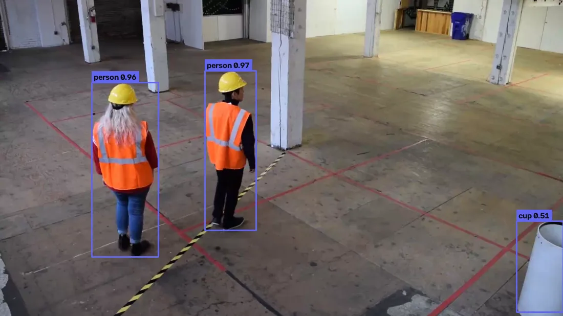
modern-yolonas predictions on a work-zone frame: two workers detected at 0.96 and 0.97, and a white pipe misread as a cup at 0.51

That frame is worth a second look, because it shows both halves of the story. The two workers come back at 0.96 and 0.97 with tight boxes, in poor indoor light, from a model running on a CPU. The white pipe on the right comes back as cup 0.51, which it plainly is not. At a deployment threshold of 0.45 that false positive survives; at 0.6 it does not, and neither does anything else you care about here. Picking that number is the actual work of deploying a detector, and no benchmark table will pick it for you.

Limitations

The weights are still non-commercial today. Open replacements are in training, but they are not published yet, and a faithful reimplementation of the architecture does not launder the licence on Deci’s COCO checkpoints. For commercial work right now, train from scratch.

Latency is not throughput, and the power profile dominates both. Every figure in the matrix is single-stream latency: one image at a time, waiting for each result. An async pipeline with several inference requests in flight will report higher FPS on the same hardware. Worse for anyone benchmarking casually: I first measured this laptop on the powersave profile with cores pinned near 1 GHz and got 300 ms per inference at 256px on CPU. The same code on the balanced profile gives 31 ms. A 10x swing, same machine, same commit. If you are comparing detectors on a laptop, check your power profile before you trust a single number, including mine.

The accuracy numbers come from one machine. The INT8, CPU and iGPU figures in Part 1 are from my RF-DETR comparison, measured on a 12th-gen Intel laptop with an Iris Xe iGPU, at 256×256, on a 500-image COCO subset. Other hardware and other resolutions will shift them. The −2.5% versus −21% quantization gap is large enough that I would expect the direction to hold, but I have measured one machine.

Parity was proven for the architecture, not for every code path. The bit-identical result covers a forward pass on an identical input tensor for S, M and L. Training, export, quantization and the video pipeline are not covered by that comparison.

This is one person’s reimplementation. It has tests and a parity proof, but it has not been battle-tested by a community the way super-gradients was.

Reproducibility

Parameter	Value
CPU	12th Gen Intel Core i7-12700H (20 threads)
dGPU	NVIDIA GeForce RTX 3060 Laptop
iGPU	Intel Iris Xe (Alder Lake-P)
RAM / OS	31 GB · Linux 6.8.0 (Ubuntu)
Python	3.10.16 (parity, to host super-gradients) · 3.13.5 (mAP)
torch	2.13.0+cu130, identical build on both sides of the parity test
numpy	1.23.0 in the parity env (forced by super-gradients’ pin) · 2.5.2 in the mAP env
super-gradients	3.7.1, with `setuptools==80.10.2` (pinned `<81` or it will not import)
modern-yolonas	commit `3d8daba` for parity; `881fce4` or later for the mAP figures. Since 17 Aug 2026 those are also in a release: `pip install modern-yolonas==0.3.0`, which is the first version to ship the channel-order fix
Model / checkpoint	`yolo-nas-{s,m,l}.safetensors`, HF `CondadosAI/detectors` snapshot `edaed6b1`, Super Gradients Model EULA [2]
Parity inputs	15 × `torch.randn(1,3,640,640)` per variant, seed 1234, CPU, `eval()`, `no_grad()`
Precision sweep	float32 and float64 at 3 inputs each, so the ratio is comparable
mAP dataset	COCO val2017, all 5000 images
mAP tool	`pycocotools` 2.0.11 `COCOeval`, bbox, conf threshold 0.001
Commands	`python examples/parity_check.py --precision-sweep` · `python examples/bench_devices.py`
Artifacts	`output/parity.md`, `output/parity_summary.csv`, `output/latency_matrix.md`
Excluded from parity	preprocessing, NMS, training, export
Latency benchmark	model inference only (no preprocessing, no NMS), single stream, synchronous, median of 30 runs after 8 warmup runs
Runtimes benchmarked	PyTorch 2.13.0+cu130 · OpenVINO 2026.3.0 · TensorRT 11.2.1.2
INT8 calibration	NNCF PTQ, 48 real frames from the demo clip, preprocessed exactly as inference does
TensorRT INT8	not measured — TRT 11 removed the INT8 calibrator API; it needs a QDQ ONNX, which I did not build
Power profile	balanced/efficient, not powersave (see Limitations)
HUD clip	Intel IoT DevKit `worker-zone-detection.mp4`, CC BY 4.0, frames 2140+, every 3rd frame, 900px

References

[1] Deci AI. super-gradients (PyPI release history; latest 3.7.1, 2024-04-08). PyPI release history

[2] Deci AI. Super Gradients Model EULA (YOLO-NAS weights licence). LICENSE.YOLONAS.md

[3] Ding, X., Zhang, X., Ma, N., Han, J., Ding, G., Sun, J. RepVGG: Making VGG-style ConvNets Great Again. CVPR, 2021. arXiv:2101.03697

[4] Chu, X., Li, L., Zhang, B. Make RepVGG Greater Again: A Quantization-aware Approach. 2022. arXiv:2212.01593

[5] Li, X., Wang, W., Wu, L., Chen, S., Hu, X., Li, J., Tang, J., Yang, J. Generalized Focal Loss: Learning Qualified and Distributed Bounding Boxes for Dense Object Detection. NeurIPS, 2020. arXiv:2006.04388

[6] Feng, C., Zhong, Y., Gao, Y., Scott, M. R., Huang, W. TOOD: Task-aligned One-stage Object Detection. ICCV, 2021. arXiv:2108.07755

[7] Szeliski, R. Computer Vision: Algorithms and Applications, 2nd ed. Springer, 2022. §6.3 (Object detection). szeliski.org/Book

[8] Xu, S., Wang, X., Lv, W., Chang, Q., Cui, C., Deng, K., et al. PP-YOLOE: An evolved version of YOLO. 2022. arXiv:2203.16250

Tagged