Find, Measure and Filter Contours in OpenCV

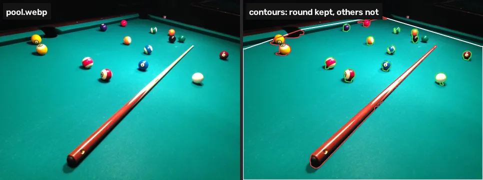
A contour is the outline of one white blob in a mask, and OpenCV can measure each outline’s size and shape, which is how the balls are told apart from the cue.

Where you have met it: Analyze Particles in ImageJ and Fiji, which counts cells or grains with a size and a circularity filter; the blob tools in machine-vision inspection software that count parts on a conveyor; coin-counting apps.

TL;DR. Once a mask has one white blob per object, OpenCV can trace each blob’s outline and measure it, so objects can be kept or thrown out by size and shape. On the pool table 14 outlines are found; 11 are round enough to be a ball, and the cue, at roundness 0.12 where a circle scores 1, is not one of them.

The problem

Lesson 3 left a clean mask with 14 blobs, and borrowed three lines to find the table. This lesson explains those lines, then turns blobs into a list of balls for the project: where each one is and whether it is round.

The table is the biggest contour

cv2.findContours traces the boundary of every white region in a mask and returns each as a list of points [1]. The cloth mask from lesson 2 has one large region, the table:

import cv2
import numpy as np

img = cv2.imread("pool.webp")
hsv = cv2.cvtColor(img, cv2.COLOR_BGR2HSV)
cloth = cv2.inRange(hsv, (75, 80, 40), (100, 255, 255))
cs, _ = cv2.findContours(cloth, cv2.RETR_EXTERNAL,
                         cv2.CHAIN_APPROX_SIMPLE)
biggest = max(cs, key=cv2.contourArea)
hull = cv2.convexHull(biggest)
print(len(cs), "contours; biggest", cv2.contourArea(biggest))
print("hull corners:", len(hull))

4 contours; biggest 571460.0
hull corners: 14

The cloth’s outline has notches wherever a ball sits against the cushion and where the pockets cut in. The convex hull stretches across the notches, so a ball against the rail is inside the table instead of on its edge [1] [3]. Filling the hull and pulling it in by the cushion’s width gives the table mask:

table = np.zeros_like(cloth)
cv2.fillPoly(table, [hull], 255)
table = cv2.erode(table, np.ones((19, 19), np.uint8))
objects = cv2.bitwise_and(cv2.bitwise_not(cloth), table)
k5, k7 = np.ones((5, 5), np.uint8), np.ones((7, 7), np.uint8)
objects = cv2.morphologyEx(objects, cv2.MORPH_OPEN, k5)
objects = cv2.morphologyEx(objects, cv2.MORPH_CLOSE, k7)
cs, _ = cv2.findContours(objects, cv2.RETR_EXTERNAL,
                         cv2.CHAIN_APPROX_SIMPLE)
print(len(cs), "contours on the table")

14 contours on the table

Measure each one

A ball seen from any angle is a disc, and a disc is as round as a shape gets. A number for “round” comes from comparing the area with the perimeter: a circle of radius r has area πr² and perimeter 2πr, so 4π × area / perimeter² is exactly 1 for a circle and smaller for anything else. A long thin cue scores close to 0.

def roundness(c):
    # 1.0 for a circle, near 0 for a stick
    area = cv2.contourArea(c)
    return 4 * np.pi * area / cv2.arcLength(c, True) ** 2

for c in sorted(cs, key=cv2.contourArea, reverse=True):
    a = cv2.contourArea(c)
    print(f"area {a:6.0f}   roundness {roundness(c):.2f}")

area  20810   roundness 0.12
area   4588   roundness 0.23
area   1773   roundness 0.82
area   1526   roundness 0.77
area   1444   roundness 0.66
area   1213   roundness 0.18
area   1165   roundness 0.63
area   1056   roundness 0.76
area    921   roundness 0.83
area    823   roundness 0.86
area    671   roundness 0.69
area    661   roundness 0.83
area    128   roundness 0.65
area     47   roundness 0.62

cv2.arcLength(c, True) is the perimeter, with True meaning the outline is closed [2]. The largest contour, about 20,800 pixels at roundness 0.12, is the cue. The next two, at 0.23 and 0.18, are clumps: the two yellow balls with the pocket behind them, and the red ball at the far end with a strip of cushion. The single balls sit between 0.66 and 0.86, and the orange and black balls, which touch, make one blob at 0.63. The two smallest are the white pieces of the green-striped ball, whose green stripe is the colour of the cloth.

Keep the round ones

Python · OpenCV Reset ▶ Run

out = img.copy()
balls = []
for c in cs:
    if cv2.contourArea(c) >= 45 and roundness(c) > 0.55:
        (x, y), r = cv2.minEnclosingCircle(c)
        balls.append((round(x), round(y)))
        cv2.circle(out, (int(x), int(y)), int(r) + 4, (0, 255, 0), 2)
print(len(balls), "balls:", balls)
cv2.imshow("round blobs", out)

Output

11 balls: [(792, 316), (425, 301), (572, 263), (347, 253), (896, 221), (593, 197), (507, 162), (688, 144), (624, 118), (608, 122), (412, 110)]

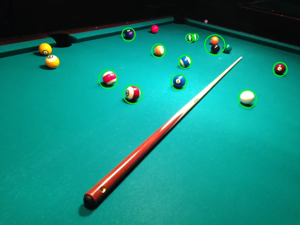
cv2.minEnclosingCircle returns the smallest circle around a contour, which gives each ball a centre and a radius [2]. Eleven blobs pass. By eye, eight are single balls, one is the orange and black balls counted as one, and two are the two white pieces of the green-striped ball. The green ball beside them is not there at all, because it is the colour of the cloth (lesson 1 read its hue at 82). Lesson 5 scores the result against a hand count on all three photos and fixes what it can.

To try a photo of your own table, press “Use your image” on the first cell of this page, then Run on this one. A cloth of another colour needs its own hue range, read as in lesson 1.

Break it

Filter on size alone and everything large enough passes:

Break it Reset ▶ Run

big = [c for c in cs if cv2.contourArea(c) >= 45]
print("kept by area alone:", len(big))
cv2.imshow("all blobs", cv2.drawContours(img.copy(), big, -1, (0, 0, 255), 2))

Output

kept by area alone: 14

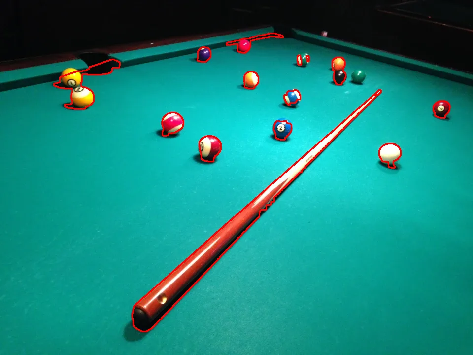
All 14 pass, including the cue and the two clumps. Size says how much of something there is; only shape says what it is.

Your turn

The cue is the largest contour on the table. Store its roundness in r.

r = None  # replace this line
print(r)

Why this works

A contour is the boundary of a connected region of white pixels, and OpenCV finds it by following the edge of each region around [3]. Area and perimeter are two of the basic descriptors of a region’s shape [4], and the roundness above combines them so that the result does not depend on how big the object is in the photo, which matters when a ball near the camera covers three times the area of one at the far end. The convex hull is itself a standard morphological construction [4]. The Fundamentals unit on binary images (2.2) is planned; until it is written, Gonzalez and Woods is the reference.

Common mistakes

• Black objects on a white background. findContours traces white regions. Invert the mask first [3].
• RETR_TREE or RETR_LIST when you only want objects. They also return the outlines of holes inside each object, which then get counted as objects. RETR_EXTERNAL returns only the outer ones.
• Filtering on area alone. The Break it cell keeps the cue. Add a shape test.
• A roundness threshold near 1. A real ball’s outline is jagged at pixel scale and often clipped by a highlight or its shadow; here single balls score 0.66 to 0.86. Leave room.

References

[1] OpenCV. Contour Features (Python tutorial, doc/py_tutorials/py_imgproc/py_contours/py_contour_features/py_contour_features.markdown). OpenCV 4.11.0, commit 31b0eee. github.com/opencv/opencv

[2] OpenCV. imgproc.hpp, documentation of arcLength and minEnclosingCircle (modules/imgproc/include/opencv2/imgproc.hpp). OpenCV 4.11.0, commit 31b0eee. github.com/opencv/opencv

[3] OpenCV. Contours: Getting Started (Python tutorial, doc/py_tutorials/py_imgproc/py_contours/py_contours_begin/py_contours_begin.markdown). OpenCV 4.11.0, commit 31b0eee. github.com/opencv/opencv

[4] Gonzalez, R. C., & Woods, R. E. (2018). Digital Image Processing (4th ed.), section 12.4 “Region Feature Descriptors”, Some Basic Descriptors, p. 982, and section 9.5 “Some Basic Morphological Algorithms”, Convex Hull, p. 715. Pearson.

[5] MarkBuckawicki. Billiards table 2.JPG (27 Feb 2014). Wikimedia Commons, CC0 1.0. commons.wikimedia.org